B. Racine, R. Flauger
Posting describing the plots and tables that will end up in the DSR, as well as the assumptions made for these results. Might change as we finalize the DSR.
Following the work done for the Science book and the Concept Definition Task Force report (CDT), we are here detailing the new iteration of forecasting made for the Decadal Survey Report (DSR). This builds on the most recent instrumental design, and introduces more realistic observation strategies.
In this posting, we introduced an update to the framework used for the previous iterations, that incorporated a new hitcount map rescaling of the bandpower covariance matrix. In this posting, we proposed some \(\sigma(r)\) vs. \(r\) plots for the DSR, using more optimal scalings. In a subsequent posting, we updated our results with a more realistic handling of the joint Pole and Chile observations, and studied the effect of the 20GHz channel on the constraints. We also tried to naively boost the foreground level in the shallow part of the Chile map, since it is hitting a region with more foreground. In a later posting, we applied a mask to the hitmap used for the Fisher forecast (thus reducing the number of modes used in the high foreground regions.)
In the current posting, we summarize what assumptions went into the DSR version, and present the 3 plots that are in the appendix A.
For the DSR, we are using the performance based Fisher forecasting framework, developed by Victor Buza, Colin Bischoff, and John Kovac, as described for instance in this posting.
We are here using information derived from the BK14 sims. Victor's posting as much more detail about these inputs.
In particular, the noise model used for the SAT tubes is directly scaled from the noise bandpowers at 95GHz (for 95GHz and below) and 150GHz (for 145GHz and above). For illustration, similar noise bandpowers for BK15, are plotted and fitted in this posting. The 20GHz channel is still based on the 95GHz data, but modified to have a \(\ell_{\rm knee}\) of 200.
The inputs also contain information about the actual map noise achieved from multiple receiver-years at {95, 150, 220} GHz, including the real penalties for detector yield, distribution of detector performance, weather, and observing efficiency.
Another very important aspect is that we are using the bandpower covariance matrix (noise only, signal only and signal x noise terms). These inputs fold in the incomplete mode coverage due to sky coverage, scan strategy, beam smoothing, and filtering in data analysis.
This is a major difference with forecastings that only take into account the filtering as a 1/f component only.
(note that for 220 and 270, we use a noise bandpower and BPCM from 150GHz, but we scale from the map noise at 220GHz achieved in 2015. As one can see in this same posting, the bandpower shape is really similar. In the next iteration, we should switch fully to the 220GHz achieved performance.)
In order to scale the BK noise bandpowers and the bandpower covariance matrix, we specify an instrument, in terms of beam, numbers of detectors, NET of these detectors etc.
The current DSR reference design for the SAT is a 18 tubes configuration, slightly updated since the post-CDT spreadsheet, is shown in this SAT spreadsheet.
We now use now [2,2,6,6,6,6,4,4] tubes, each with [288, 288, 3524, 3524, 3524, 3524, 8438, 8438] detector per tube on a SAT for [30, 40, 85, 95, 145, 155, 220, 270] GHz, and 135 detectors at 20GHz on a LAT (with FWHM of 11 arcminutes and a NET of 214 \(\muK\sqrt{s})).
This configuration was basically a possible realization of the CDT strawperson design, as was investigated in spreadsheet.
In the following tables, as well as in figure 3, we also use the other configurations: 6 (1,2,2,1), 9 (1,3,3,2), 12 (1,4,4,3), 18 (2,6,6,4), and 30 (2,10,10,8) where this notation shows the dichroic coupling. These configurations have been chosen so that they can sum to the default 18 tubes, but over 2 sites (except for the 30 tubes case of course).
Note that since the 20GHz channel is on the delensing LAT, it is only able to observe the patches that will be delensed, i.e. not in the shallow Chile one (see later). Previously we had ignored that fact and were rescaling the 20GHz channel for the Chile observations in the same way as from Pole. We are now accounting for the fact that there is only one 20GHz tube, at Pole. Note that we also take into account that if all the SATs are in Chile, we can still use the 20GHz from Pole on the deep delensed patch.
For the BB signal, we consider a 12 parameter model, with a CMB+lensing component, a dust modified black body emission and a synchrotron power law emission. The parameters used are shown in table 1.
| Parameter | Description | Value |
|---|---|---|
| \(r\) | tensor-to-scalar ratio | [0,0.003,0.01,0.03] |
| \(A_L\) | lensing amplitude | Input from delensing optimization |
| \(A_\mathrm{dust}\) | polarized dust amplitude, at 353 GHz and \(\ell = 80\) | 4.25\({}^*\) \(\mu\mathrm{K}_\mathrm{CMB}^2\) |
| \(\beta_\mathrm{dust}\) | polarized dust frequency spectral index | 1.59 |
| \(\alpha_\mathrm{dust}\) | polarized dust spatial spectral index | -0.42 |
| \(\Delta_\mathrm{dust}\) | polarization dust decorrelation parameter | 0.97 or 1 |
| \(T_{dust}\) | dust greybody temperatur | 19.6K |
| \(A_\mathrm{sync}\) | polarized synchrotron amplitude, at 23 GHz and \(\ell = 80\) | 3.8\({}^*\) \(\mu\mathrm{K}_\mathrm{CMB}^2\) |
| \(\beta_\mathrm{sync}\) | polarized synchrotron frequency spectral index | -3.1 |
| \(\alpha_\mathrm{sync}\) | polarized sync spatial spectral index | -0.60 |
| \(\Delta_\mathrm{sync}\) | polarization sync decorrelation parameter | 0.9999 or 1 |
| \(\epsilon\) | sync/dust spatial correlation parameter | 0 |
The decorrelation remapping function is now as described in appendix F of BK15. Note that we are still using a quadratic \(\ell\)-dependence, as introduced in Victor's posting and used for the CDT report and the science book.
One of the main changes since the last iteration of forecasts, which used a simple constant rescaling of 3 ot 20 to take into account the observation of larger patches with respect to the current BK patch, is that we now use more realistic sky coverages, introduced in these postings: Pole wide, Pole deep and Chile deep.
A plot of the hitmaps corresponding to these strategies is shown in figure 7 of posting.
The main effect to take into account for these more complex strategies is the fact that the noise and signal degrees of freedom are affected in different ways, so we will need to recale the different terms of the bandpower covariance matrix individually.
These rescalings depend on the way we analyse our data. In BK, to compute the bandpowers, we use an inverse noise variance weighting. Here, in some cases the signal (\(r\) + residual lensing + foreground residuals) will be dominating, so we need to take this into account for optimal weighting.
These scalings are presented in Appendix A of this posting.
Foreground bias.
In this posting, we are using the BK foreground minimum at ell=80 as an estimate of the foregrounds amplitude
and translating this into a \(r\)-equivalent.
We then extrapolated it to the Chile observing strategy; for that we assume that the scaling was well described by what we got from map based analysis for the fitted \(A_{fg}\) for the 04b and 04c hitmaps, model 7 having supposedly the most data-driven realistic foreground variation.
We then used the more complex models to back up the fact that unmodeled foreground will leave a bias on \(r\) that will linearly depend on the foreground amplitude.
Here we consider the fg residual to be 1% of the total foreground, which is of course a “soft” choice, and add it in quadrature to \(\sigma(r)\).
This is a crude estimate and should be improved in future iterations of the forecasting exercise.
Observation efficiency penalty.
We also consider a case for the tables, where the observing efficiency in Chile is half that at Pole. This is done by multiplying the noise spectra by 2. Once we have high sensitivity maps delivered from Chile, we will of course update our performance based inputs and won't rely on these choices.
For the DSR, we want to compare \(\sigma(r)\) for different observing strategies, for different levels of \(r\), using SATs with 18 tubes, as described in this SAT spreadsheet, as well as a "delensing" survey at Pole, and the two LATs in Chile.
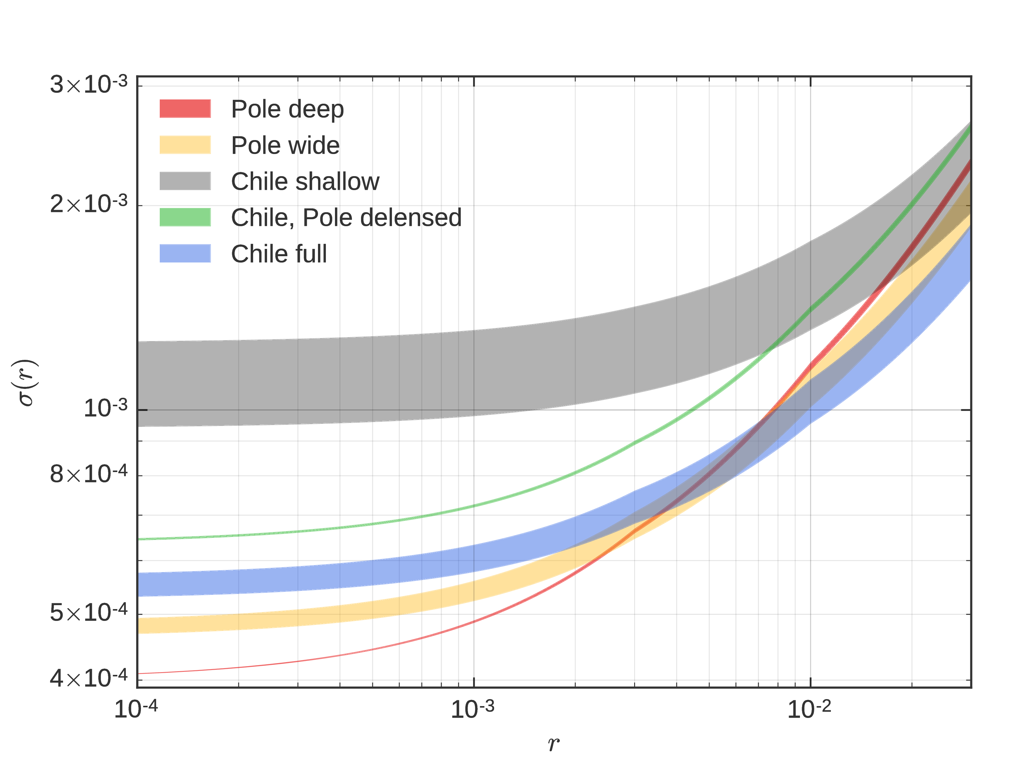
For the following figures, we computed the residual optimal \(A_{\rm delens}\) achievable using the LATs. For the Chile narrow case, we split the observations into a deep patch, which overlaps fully with the Pole deep patch and is delensed by the "delensing" LAT at Pole, and the shallow part, which is delensed by the Chile LATs. For the Pole strategies, we use the "delensing" survey.
In the Chile case, we combine the shallow and deep part of the observations into the "Chile full" constraints, by adding them in quadrature.
In figure 3, we show combined observations, where we computed the scalings and the \(A_{\rm delens}\) for the sum of the hitmaps, to mimick a joint analysis of the datasets. We then add the shallow patch constraints in quadrature.
Note that for these figures, we show the linear interpolation of \(\sigma(r)\) from the 4 computed cases: \(r=0,0.003, 0.01, 0.03\).
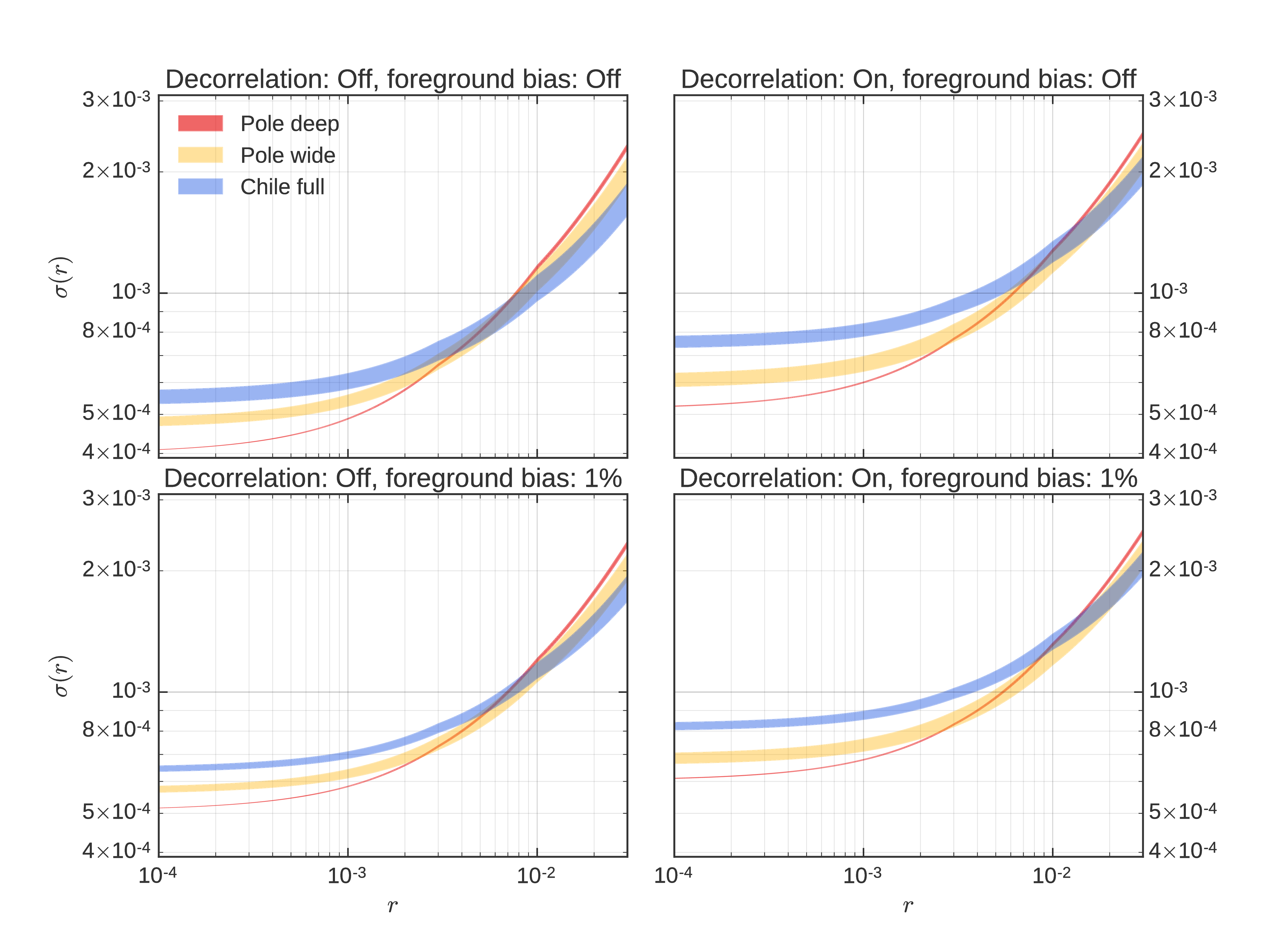

The tables for the DSR contain forecasted \(\sigma(r)\) for different sitings. The first row represents the Pole only constraints. We consider both Pole wide and Pole deep strategy, and take the best case. In the case where we have a strong signal, it is better to go slightly wider, as can be seen in Figure 2 for instance. The first column represents the Chile only constraints. Here we use the Chile full constraints, i.e. the quadrature sum of the deep, Pole delensed part and the shallow, Chile LAT delensed part, of the chile narrow hitmap. For the cross terms, we use the combined Pole delensed observing strategy constraints, to which we add the Chile delensed constraints in quadrature. We highlight the combinations that sum to 18 tubes in bold.
We also present the 95%CL limit in the case where \(r=0\) and the significance of detection in the case where \(r=0.003\). Remember that our goal is 0.001 at 95CL and 0.003 at \(5 \sigma\).
Since the output of the Fisher framework is \(\sigma(r)\), we need a way to convert these into our final statistics, taking into account the fact that the likelihood is non-Gaussian. Colin introduced an Ansatz for that step in this posting.
Here we use that Ansatz to compute the marginalized \(r\) likelihood for every single Fisher case. We compute the 95%CL using the cumulative sum of the likelihood, and the significance of detection using the 0-to-peak ratio. When we combine the pole delensed observations with the LAT delensed ones, we take the product of the 2 likelihoods and calculate our statistics. Here we make the approximation that the number of degrees of freedom (k in Colin's posting), just scales with \(f_{\rm sky,noise}), with respect to the parameter fitted by Colin for the B3 hitmap. The residual foregrounds and lensing signal have a small effect, as was already visible in his posting.
Note that these statistics correspond to a case where the signal in our patch peaks exactly at \(r=0\) or \(r=0.003\). Of course, a given realization of the a \(r=0.003\) sky, the likelihood will peak at different values. One would want to then simulate this sample variance and compute the significance of detection and 94%CL for a bunch of simulation and report the median value. This is for now defered to future work.
Since the CDT, we introduced more realistic observation strategies, but there are other approximations to keep in mind when interpreting our results :