Fisher projections for CMB-S4, v3

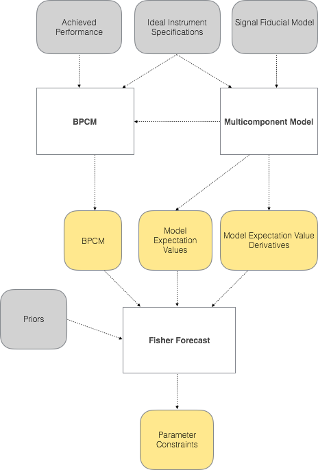
This posting describes the development of a Fisher forecasting framework (developed by Victor Buza, Colin Bischoff, and John Kovac), specifically targeted towards optimizing tensor-to-scalar parameter constraints in the presence of Galactic foregrounds and gravitational lensing of the CMB. I first describe the methodology and then present an example forecast for CMB-S4.

1. Schematic of Fisher Machinery

Figure 1 is a schematic representation of the framework, indentifying the user inputs, code modules, and outputs of said modules. This code overlaps significantly with the code used for the BICEP/Keck likelihood analysis and our belief in the projections is grounded in that connection to achieved performance / published results. In particular, we emphasize the importance of using map-level signal and noise sims (of the BICEP2/Keck dataset) as a starting point. We know that these sims are a good description of our maps because we pass jackknife tests derived from them.

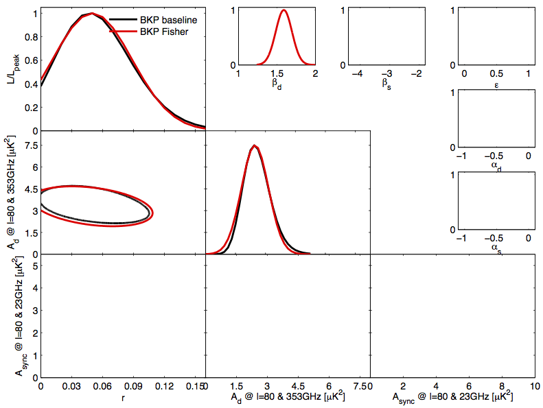
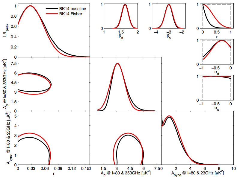
Our confidence in these projections is further enhanced by their ability to recover achieved parameter constrains quoted in the BKP and BK14 papers. BK14 quotes an achieved \(\sigma_r=0.024\) by performing an 8-dimensional ML search (with priors) on a set of 499 Dust + \(\Lambda\)CDM sims, and deriving the standard deviation of the recovered \(r_{ML}\). Though BKP did not do a similar exercise, were it to do that, it would have quoted \(\sigma_r=0.032\). Our Fisher forecasts for these particular scenarios recover \(\sigma_r=0.033\) and \(\sigma_r = 0.024\), which are within sample variance (from the finite number of sims) from the real results. For the particular data draws of BKP and BK14, we can even compare the marginalized posteriors to the Fisher Contours, though this is a weaker comparsion. Firstly, we know the Fisher Contours will be Gaussian, while the real contours will likely not (BKP and BK14 use the H-L likelihood approximation), and secondly, we know that each particular data realization will yield differently shaped contours, so an ideal match of Fisher Contours to any particular realization should not be expected. Nonetheless, the contours are still quite faithfully recovered: BKP vs Fisher, BK14 vs Fisher.

Inputs

• Achieved Performance:The code takes information derived from signal and noise sims of the BK14 dataset (could be adapted to use similar information from another experiment). More specifically, we use signal-only, noise-only, and signal x noise bandpower covariance terms, as well as the ensemble-averaged signal and noise bandpowers. These inputs contain information about the actual map depth achieved from X rx-years at 150 GHz + Y rx-years at 95 GHz, including the real penalties for detector yield, distribution of detector performance, weather, and observing efficiency. These inputs also fold in the incomplete mode coverage due to sky coverage, scan strategy, beam smoothing, and filtering in data analysis. For projections, we assume that we can scale down the noise based on increased detector count and integration time (note that this requires the assumption that detector noise is uncorrelated and we don't suffer heavily from common-mode atmospheric noise) and that we can apply beamsize rescaling to estimate performance at other frequencies.


• Instrument Specifications: Number of frequencies and bandpass data specifying observing frequency response for each experiment included in the analysis, beamsize ("Achieved Performance" inputs fold in the actual BICEP/Keck \(B_l\), but we rescale based only the Gaussian beamwidth), Bandpower Window Functions (but the bandpower covariance inputs of "Achieved Performance" have only been calculated for the BICEP/Keck bandpower definitions), Number of detectors per each frequency, and ideal per-detector NET's per each frequency. From the last two items, we can make an idealized calculation of the instrument sensitivity. This "ideal instrument sensitivity" is compared to the ideal sensitivity of BICEP/Keck to calculate the noise scaling factors. Applying these factors to the achieved sensitivities of BICEP/Keck yields achieved sensitivities in our new bands.


• Signal Fiducial Model: Parameters used to calculate the multicomponent model. Our standard model has twelve parameters, discussed below. For the example projection included in this posting, we choose the foreground parameters to the best-fit values from BK14 (\(A_{dust} = 4.25 \mu\mathrm{K}_\mathrm{CMB}^2\), \(A_{sync} < 3.8 \mu\mathrm{K}_\mathrm{CMB}^2\) (at 95%)). We consider two options for tensors, r=0 or r=0.01. Currently, delensing is included in the forecasts by choosing \(A_L\) < 1 in the fiducial model (thereby reducing the lensing sample variance). We consider the fixed values \(A_L\) = {1, 0.5, 0.2, 0.1, 0.05, and 0}, as well as letting \(A_L\) be a dynamic variable.

Multicomponent Model

• Parametrized model of one or more signal fields, including how the different signals scale to the various observing frequencies. Our model includes four signal components: a CMB component, parametrized by r and A_L, and components of uncorrelated dust, uncorrelated synchrotron, and correlated dust and synchrotron (which has a frequency scaling that depends on the relative strength of dust and sync). This description is the same as having a spatially independent CMB component, and partially correlated dust/sync. We assume that the synchrotron scales as a simple power law in both frequency, and ell, while for Dust we assume a power law scaling in ell, and a greybody SED for the frequency dependence. While this model is easily extendable, other models could be substituted here.

• The twelve parameters defining our model are:

  1. \(r\), tensor-to-scalar ratio
  2. \(A_L\), lensing amplitude
  3. \(A_\mathrm{sync}\), polarized synchrotron amplitude, in \(\mu\mathrm{K}_\mathrm{CMB}^2\), at 23 GHz and \(\ell = 80\).
  4. \(A_\mathrm{dust}\), polarized dust amplitude, in \(\mu\mathrm{K}_\mathrm{CMB}^2\), at 353 GHz and \(\ell = 80\).
  5. \(\beta_\mathrm{sync}\), polarized synchrotron frequency spectral index
  6. \(\alpha_\mathrm{sync}\), polarized synchotron spatial spectral index
  7. \(\beta_\mathrm{dust}\), polarized dust frequency spectral index
  8. \(\alpha_\mathrm{dust}\), polarized dust spatial spectral index
  9. \(E/B\) ratio for sync (value of 1 implies equal power in \(E\) and \(B\))
  10. \(E/B\) ratio for dust (value of 1 implies equal power in \(E\) and \(B\))
  11. \(\epsilon\), sync/dust spatial correlation parameter
  12. \(T_{dust}\), dust greybody temperature


• In Section 5, I introduce a 13th parameter, modeling dust decorrelation, and show its effects on the constraints of our parameters of interest.


• Since each signal component is independent, they have zero-cross power. So for a given spectra, the code just steps through the model components, combines the appropriate amplitude functions for the two experiments contributing to the spectrum, and applies the bandpower window functions to get the binned expectation values. Finally, it sums over model components to get the total expectation value for that spectrum. In addition, since a Fisher Forecast requires knowledge about the response of the model expectation values with respect to the model parameters, the code also outputs the derivatives of the model expectation values.

BPCM (Bandpower Covariance Matrix)

• Signal Scaling:
  The output model expectation values can also be useful in the formation of our bandpower covariance matrix. For the multicomponent analysis, we have been using lensed-LCDM + \(A_{dust}\)=3.75 (signal + noise) sims to construct the bandpower covariance matrix components. But, because we have the individual signal-only, noise-only, and signal x noise terms, we can record all the bpcm components:

  1. sig = signal-only terms of the form \(\mathit{Cov}(S_i \times S_j, S_k \times S_l)\)
  2. noi = noise-only terms of the form \(\mathit{Cov}(N_i \times N_j, N_k \times N_l)\)
  3. sn1 = signal×noise terms of the form \(\mathit{Cov}(S_i \times N_j, S_k \times N_l)\)
  4. sn2 = signal×noise terms of the form \(\mathit{Cov}(S_i \times N_j, N_k \times S_l)\)
  5. sn3 = signal×noise terms of the form \(\mathit{Cov}(N_i \times S_j, S_k \times N_l)\)
  6. sn4 = signal×noise terms of the form \(\mathit{Cov}(N_i \times S_j, N_k \times S_l)\)

  and then rescale and combine them to create a bandpower covariance matrix for a new desired multicomponent model. Here, \(S\) are signal sims, \(N\) are noise sims, and the indices \(i,j,k,l\) run over fields in the analysis, i.e. all combinations of a map type (\(T, E, B\)) and an experiment (BK, P353, etc.). For many combinations of indices, we set certain covariance terms to be identically zero—\(\mathit{Cov}(N_{BK} \times N_{BK}, N_{P353} \times N_{P353})\), for example. It is worth noting that having all of these terms allow us to have different number of degrees of freedom per bandpower for noise than for signal, a complication that is often ignored in other analyses by setting the noise and signal degrees of freedom to be identical.

  While calculating the covariances from the signal and noise sims, we record the average signal bandpowers from the sims. For a new signal model, we can calculate the new bandpower expectation values, and rescale the signal components in the bandpower covariance matrix by the appropriate power of the ratio of the recorded average signal bandpowers, and the newly calcualted expectation values.

  The ability to get a BPCM for any model is a great one to have, because it means you don't have to run sims for any and all concievable scenarios, all you need is one set of sims. I should emphasize that we only apply this step once in our process; we do not rescale our BPCM at every step of the way.

• Noise Scaling:
  In addition to scaling from one signal model to the other, recording all of the covariance terms allows us to rescale the noise parts as well. Given a dataset for which we have sims, the noise scaling can go one of two ways: the first allows one to take a frequency present in the dataset and scale down the noise in the BPCM by the desired amount; the second one allows one to add an additional frequency by taking an existing one, scaling down the noise by the desired amount, and then expanding the BPCM and filling it in with the appropriate variance and covariance terms between this new band, and all of the old ones. These two tools allow us to set up a new data structure to explore any combination of frequency bands, with any sensitivity in each band.

  We would like to base our noise scaling factors on achieved sensitivities rather than ideal performances. To that end, we use the achieved survey weights (of BICEP/Keck: {95, 150, 220}) to obtain projected weights for any of the S4 channels.

  We can write the survey weight as follows: \[w_{achieved} = \frac{t_{obs}}{\alpha_{\frac{ideal}{achieved}} NET^2_{ideal}}\] where \(\frac{t_{obs}}{\alpha_{\frac{ideal}{achieved}}}\) encapsulates the less-than-ideal observing time, receiver perfomance, cuts, etc. It is the factor that takes us from the ideal scenario to reality. Then, to obtain the survey weight at a new frequency, simply calculate: \[w_{\nu_2,achieved} = w_{\nu_1,achieved} \frac{NET^2_{\nu_1, ideal}}{NET^2_{\nu_2,ideal}}\] The implicit assumption that is made here is that the reality factor for this new frequency is exactly the same as the one from which we are scaling. To not abuse this assumption, the survey weight scaling is always done from the closest frequency that we have an achieved survey weight for, as that is the perfomance that should guide us.

  Now, to get \(N_l\)'s at a new frequency by scaling the \(N_l\) from an existing frequency, in addition to scaling them by the ratio of the survey weights, I must note that in our sim pipeline, in applying suppression factors, both the signal and the noise parts of the sims are scaled by the beam of the respective frequency they are calculated for. Therefore, to obtain \(N_l\)'s for one channel by scaling the achieved \(N_l\)'s of another channel, we have to reapply the beam of the second, and scale back by the beam of the first. Under the assumption of Gaussian beams, we can write the full scaling as: \[N_{l,\nu_2} = N_{l,\nu_1} \frac{w_{\nu_1,achieved}}{w_{\nu_2,achieved}} \frac{B^2_{l,\nu_2}}{B^2_{l,\nu_1}}\] where \(B^2_{l} = \exp(-\frac{l(l+1)\theta^2}{8log(2)})\), and \(\theta\) is the FWHM (in radians) of the Gaussian beam. With the \(N_l\)'s scalings on hand, we can perform the above mentioned BPCM operations to arrive at a BPCM that encompasses the intricacies of reality.

Fisher Forecast

• Given a Likelihood function of the form: \[ \mathcal{L(\theta; d)} \sim \frac{1}{\sqrt{det(\Sigma(\theta))}} exp\{ -\frac{1}{2}(d-\mu(\theta))^T \Sigma(\theta)^{-1} (d-\mu(\theta)) \} \] where \(d\) is the data, \(\theta\) are the theory parameters, \(\mu(\theta)\) are the expectation values given the parameters, and \(\Sigma(\theta)\) is the bandpower covariance matrix, which can also be a function of the parameters. We can introduce the Fisher Information Matrix definition: \[ F_{ij} = -<\frac{\partial^2 log(\mathcal{L(\theta; d)})} {\partial\theta_i\partial\theta_j} > \] which is simply the average of the log-likelihood curvature. After some algebraic manipulations we can arrive at: \[ F_{ij} = \frac{\partial\mu^T}{\partial\theta_i} \Sigma^{-1} \frac{\partial\mu}{\partial\theta_j} + \frac{1}{2} Tr( \Sigma^{-1} \frac{\partial\Sigma}{\partial\theta_i} \Sigma^{-1} \frac{\partial\Sigma}{\partial\theta_i}) \] Previous studies of the BK14 \(\sigma_r\) stastic, derived as the standard deviation of the recovered ML values for r from an N-dimensional ML search on Dust + \(\Lambda CDM\) sims, has shown that it is best recovered with a Fisher formulation for which \(\Sigma(\theta) = \Sigma\), thus sending the second term to zero. In all the projections below we abide by these findings, and continue to calculate only the first term of Fisher, though the code is set up to allow one to calculate either of the terms.


• Priors: If we have prior knowledge of a given parameter \(\theta_i\), we can easily introduce this information into the Fisher Matrix. Simply add \(P_i=1/\sigma_i^2\) to the diagonal of the Fisher Matrix, where \(\sigma_i\) is the width of the prior. By extension, you can do a similar step if you want to just completely fix the parameter -- fixing a parameter would be equivalent to having a very small \(\sigma\) on that parameter, which would result in adding a very large number to the corresponding diagonal element of the Fisher Matrix. Alternatively, one can simply remove the rows and columns of the Fisher Matrix, corresponding to the parameters we want fixed. If we'd like to impose a flat prior on any parameter, adding a \(P_i=0\) has that effect by effectively having a really large \(\sigma_i\).


• Finally, we calculate our paramter constraints as \(\sigma_{\theta\theta}=\sqrt{(F^{-1})_{\theta\theta}}\)

Figure 1:

This is a schematic representation of our Fisher Machinery. Grey ovals represent User Inputs, White boxes represent Code Modules, and Yellow ovals represent Code Outputs.

2. Worked-out Example; Experiment Specification

Below, I present an application of this framework to an example motivated by previous BICEP/Keck experience.

• For this particular example I assume eight S4 channels: {30, 40, 85, 95, 145, 155, 215, 270} GHz, two WMAP channels: {23, 33} GHz and seven Planck channels: {30, 44, 70,100, 143, 217, 353} GHz.


• This example assumes BICEP3-size appertures (slightly larger than BICEP/Keck), and scales the beams accordingly.


• The assumed unit of effort is equivalent to 500 det-yrs at 150 GHz. For other channels, the number of detectors is calculated as \(n_{det,150}\times \left(\frac{\nu}{150}\right)^2\), i.e. assuming comparable focal plane area (these are roughly equivalent to current Keck receivers). The projections run out to a total of 5,000,000 det-yrs (5,000,000 det-yrs, if all at 150 GHz, would be equivalent to 500,000 detectors operating for 10 yrs -- this seems like a comfortable upper bound for what might be conceivable for S4. S4 scale surveys seem likely to be in the range of \(10^6\) to \(2.5\times10^6\) det-yrs).


• The ideal NET's per detector are assumed to be {221.4, 300.9, 300.6, 275.5, 337.7, 373.1, 699.6, 1313.8} \(\mu\mathrm{K}_\mathrm{CMB}^2 \sqrt{s}\). I emphasize again that these numbers are only used to determine the scalings between different channels, and NOT to calculate sensitivities. All sensitivities are based on achieved performance.


• The BPWF's, ell-binning, and ell-range are assumed to be the BICEP/Keck ones; yielding 9 bins with nominal centers at ell of {37.5, 72.5, 107.5, 142.5, 177.5, 212.5, 247.5, 282.5, 317.5}.


• The Fiducial Model for the Fisher forecasting is centered at either \(r\) of 0 or 0.01, with \(A_{dust} = 4.25\) (best-fit value from BK14) and \(A_{sync}=3.8\) (95% upper limit from BK14). The spatial and frequency spectral indeces are centered at \(\beta_{dust}=1.59, \beta_{sync}=-3.10, \alpha_{dust}=-0.42, \alpha_{sync}=-0.6\), and the dust/sync correlation is centered at \(\epsilon=0\).


• The Fisher matrix is 8-dimensional. The 8 parameters we are constraining are: {\(r, A_{dust}, \beta_{dust}, \alpha_{dust}, A_{sync}, \beta_{sync}, \alpha_{sync}, \epsilon\)}. Where \(\beta_{dust}\) and \(\beta_{sync}\) have Gaussian priors of \(0.11, 0.30\), and the rest have flat priors.


• For delensing, I first do the same 6 levels of fixed delensing as for the first posting, and then implement delensing as an extra band in the optimization. I assume the delensing experiment has a mapping speed equivalent to the 145 channel, and then use Kimmy's calculations to go from a map noise level to an effective level of residual lensing.

3. Parameter Constraints; \(\sigma_r\) performance

In this section, I focus on the 1% BICEP/Keck patch, and search for the optimal path for a number of fixed levels of delensing. In addition, I also fold in delensing as an extra band in the optimization, thus allowing the algorithm to decide at each step if the effort is better spent towards foreground separation, or towards reducing the lensing residual. I optimize for two possible levels of tensors: \(r=0\) and \(r=0.01\), and plot the resulting paths, individual map depths in \(\mu K\)-arcmin, the effective lensing residuals (after delensing), the amount of effort spent delensing, \(\sigma_r\)'s, and logarithmic derivatives of \(\sigma_r\). In addition to the various delensing cases, I also consider a Raw Sensitivity case (conditional on zero foregrounds).

Things to note:

• Choosing "Adaptive/Optimal/r=0" we see that for our foreground model the optimal effort distribution is spread across four different frequencies, one in each of the atmospheric bands. We know that experimentally there is lots to be gained from observation in all eight frequencies, so one can click the "Force Split" button to spread the effort equally among bands in the same atmospheric window. We should recognize that the quantitative behavior of the optimal path is NET dependent, and could look somewhat different for different detector sensitivities, however, the qualitative behaviour will still holds.


• Choosing "Adaptive/Force Split/r=0" we see that at the level of \(10^6\) det-yrs, we achieve \(\sigma_r = 6\times10^{-4}\), while spending ~40% of the effort to achieve a lensing residual of 5% (in power units). For an \(r=0.01\) signal we get \(\sigma_r = 2\times10^{-3}\) for the same amount of effort, though as the logarithmic-derivative plot points out, in the case of a signal being present, after about \(10^5\) det-yrs one would gain by going to more sky rather than drilling deeper in the 1% patch assumed for this optimization. For the \(f_{sky}\) dependence see next section.


• To maximize the usefulness of the logarithmic derivative plot, we can identify three values of interest: 0, -0.5, -1.0. When the derivative is 0, it means some floor was hit and there is no improvement on \(\sigma_r\); when the derivative is above -0.5, it signifies that at that point one would gain more by going to more sky rather than acquiring more survey weight on that patch. The logic behind that is that where I to repeat the same measurements on a number of N different, yet equivalent, patches, my \(\sigma_r\) constraint would improve as \(\sqrt{N}\); thus, any logarithmic improvement that is slower than -0.5 means one gains more by going to more sky. Lastly, when the derivative is -1.0, it means one keeps gaining linearly with time, as seen in the raw sensitivity case.

Figure 2:

(Top, Left) Optimal path indicating the total number of det-yrs, and the individual distribution of det-yrs at each point.
(Top, Right) Individual map depths for every channel, in \(\mu K\)-arcmin. Calculated from the accumulated weights in each channel on the BICEP2 patch.
(Middle, Left) Ratio of the total effort that is spent on delensing, as a function of total effort.
(Middle, Right) Effective \(A_L\) as a function of total effort.
(Bottom, Left) Resulting \(\sigma(r)\) constraints for each level of delensing, as well as from a limiting (conditional on no foregrounds) raw-sensitivity case.
(Bottom, Right) The logarithmic derivative of \(\sigma(r)\) with respect to det-yrs, indicating the different regimes of gain.

• Fixed Level of lensing chooses particular fixed levels of delensing (Note: the delensing effort is then not included in the total # of det-yrs, i.e. it requires extra effort).


• Adaptive lensing allows delensing to be treated as an extra dimension in the steepest descent algorithm (therefore the delensing effort is included in the total # of det-yrs).


• Optimal path does not force any band-splitting; it purely shows the most optimal path.


• Force split makes sure the amount of effort in each band (within an atmospheric window) is equivalent. (Note: the top panels might have overlapping lines because of this; it's easy to get fooled visually).

4. \(\sigma_r\) vs \(f_{sky}\)

Our Fisher formalism also includes an \(f_{sky}\) knob. The effects of \(f_{sky}\) are implemented in two steps:

• First, inflate the \(N_l\)'s by a factor \(f_{sky}\) to take into account the redistribution of the achieved sensitivity onto a larger patch.
• Second, increase the number of degrees on freedom in the BPCM by \(f_{sky}\) to account for the fact that we are now observing more modes.

Things to note:

• For a fixed 5% delensing (at an effort of \(5\times10^5\) det-yrs), the minimum is around \(f_{sky}=0.01\), which should mean that in the pager above we should see this line have roughly a -0.5 log derivative (at an effort of \(5\times10^5\) det-yrs). This is indeed the case, and is a good intuitive check.
• Given the two effects of \(f_{sky}\) on our \(N_l\)'s and BPCM, one can convince themselves that in the noise dominated regime \(\sigma_r\) should get worse as \(\sqrt{f_{sky}}\), while in the signal dominated regime, \(\sigma_r\) should get better as \(\sqrt{f_{sky}}\). Both of these regimes can be seen in this pager (for fixed level of delensing): if you go to \(10^6\) det-yrs, and focus on the blue line as \(f_{sky}\) is tiny, you will see that the slope of the blue line is \(-0.5\), if you instead focus on the black line you will notice that the slope is \(+0.5\).
• For the adaptive (dynamic) delensing, one can see how the effective lensing residual, and the amount of effort going towards delensing, changes with \(f_{sky}\). A reasonable range for S4 is between \(10^6\) and \(2.5\times10^6\) det-yrs. You can flip between the various options to see the recovered \(\sigma_r\) levels, and the \(f_{sky}\) minimum.

There are a number of effects that penalize large \(f_{sky}\) that are not included in this analysis:

• First, the foreground treatment currently assumes equal foreground amplitudes even as we increase the sky area, whereas we know that above \(f_{sky}\) of 0.1 the foregrounds will get brighter.
• The treatment also assumes single fits for foreground parameters over the entire survey, more realistic treatment would refit the foreground parameters for smaller subregions and that will reduce the sensitivities at larger \(f_{sky}\).
• The foreground parametrization in this section does not include complexity such as decorrelation effects; this is explored in Sectin 5 of this posting.
• Similarly, no systematic penalty is imposed, and that will introduce uncertainties in the fractional residual power levels that are worse for lower map signal to noise of the large \(f_{sky}\) cases.

Figure 3:

• Accumulated weight allows one to select a number of different levels of effort.


• Fixed level lensing allows one to look at any of the six levels of fixed delensing values. As mentioned in the pager above, this assumes that these levels of delensing are achieved externally, and therefore does not factor into the optimization problem the amounts of effort it would take to achieve these levels of delensing. All of the effort is purely thrown at foreground cleaning. The optimization is done over a 1% patch, and the optimal number of det-yrs in each band for each level of effort stays constant as I vary \(f_{sky}\)


• \(f_{sky}\) reoptimized (adaptive) lensing uses the aforementioned "adaptive" method, which allows delensing to be treated as an extra dimension in the optimization, and therefore does take into account the amount of effort it takes to delens. In addition, the optimization is re-done for each \(f_{sky}\).

5. Dust decorrelation

>> Decorrelation parameterization

The correlation coefficient for a particular cross spectrum is given by the ratio of the cross-spectrum expectation values to the geometric mean of the auto-spectra (if there is a non-zero decorrelation effect, the cross will register less power than the geometric mean of the autos, R<1). Therefore, the decorrelation coefficient is given by (1-correlation): \[\tilde{R}(217,353) = 1-\frac{< 217\times 353>}{\sqrt{<217\times 217><353 \times 353>}}\] This is a quantity that is less than or equal to one, dependend on the two frequencies involved in the cross, and perhaps different for different scales. We can try to model this more generally by assuming that it has a well-behaved \(l\) and \(\nu\) dependence, reflecting the different degrees of correlation one would get at various scales for different cross spectra: \[R(\nu_1,\nu_2,l) = 1 - g(\nu_1,\nu_2) f(l)\] where \(g(\nu_1,\nu_2)\) and \(f(l)\) can take different function forms. The four fairly natural scale dependencies I have explored are: \(f(l)=al^0\), \(f(l)=al^1\), \(f(l)=alog(l)\), and \(f(l)=al^2\), where \(a\) is a normalization coefficient. I am not motivating these physically, but I will argue that they span a generous range of possible scale dependencies.

Now, for the frequency scaling, John and I came up with a more well-motivated behaviour, and it stems from one of the ways through which decorrelation could be generated. The premise is simple: given a dust map at a pivot frequency, if there is a physical phenomenon that introduces a variation(\(\Delta \beta\)) of the dust frequency spectral index map \(\beta\), when extrapolating to other frequencies, the variation we've just introduced will change the dust SED and create decorrelation effects at various frequencies. We built this toy model so that we could study the resulting frequency dependence, and we've come up with the empirical form (where \(g'\) is a normalization factor): \[g(\nu_1,\nu_2)=g'*log\left(\frac{\nu_1}{\nu_2}\right)^2\]

>> Decorrelation re-mapping and normalization choice

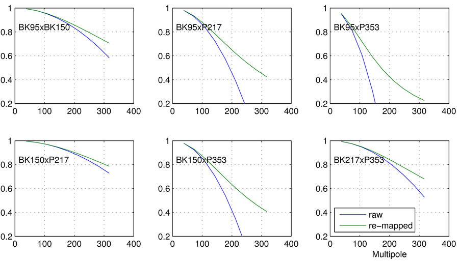
For the analysis below I define my normalization factor \(a*g'\) such that \(g(217,353)=1\) and \(f(l=80)=a\), making \(R(217,353,80)=1-a\). The reason for this normalization definition is mostly the historic over-representation of \(R(217,353,l)\) in conversations about decorrelation. In my studies, the form of \(f(l)\) (out of the ones listed above) that yields the largest decorrelation effects is unsurprisingly \(f(l)=a l^2\); therefore, as an example of an extreme case, I pick this \(f(l)\) shape, and choose my normalization coefficient to be \(a=0.03\), which PIPXXX, Appendix E says is \(1\sigma\) away from the mean decorrelation over the studied LR regions. For this particular \(a\) and \(f(l)\) choice, my correlation remapping looks (for a few of the more important cross spectra for a BK14-like analysis), like this. Notice that these are generally large values of decorrelation.

>> Effects of decorrelation in our Fisher optimization

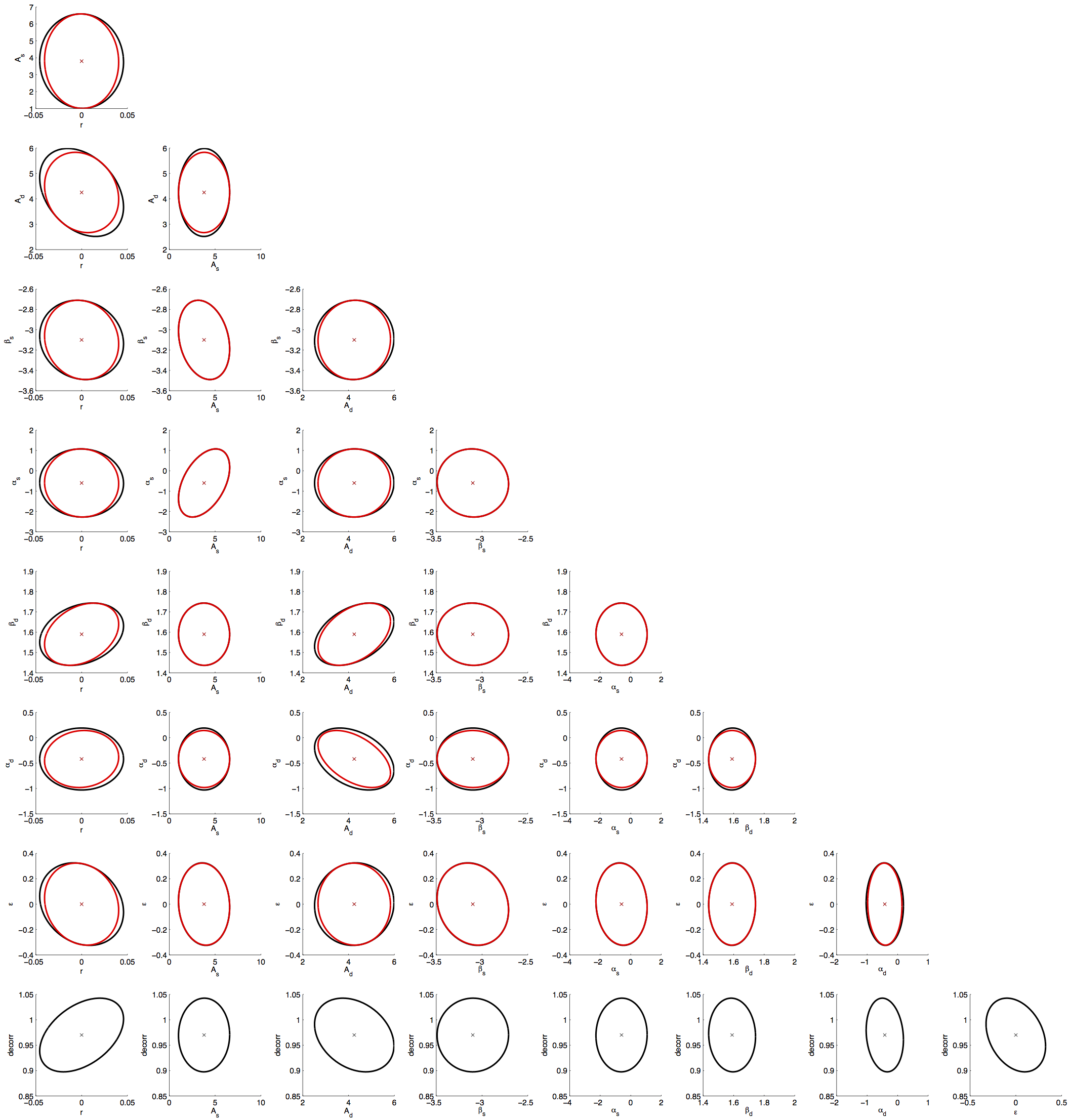
First, I would like to show an example by demonstrating the decorrelation effects for a BK14 evaluation: BK14 Fisher Ellipses with (black) and without (red) Decorrelation. You can notice the degeneracies of the decorrelation parameter with the dust parameters, as well as \(r\). In addition, this also makes it easy to observe the effects of the decorrelation on the constraints of these parameters; in particular, we see that it introduces more degeneracy in the \(r\) vs \(A_d\) plane, and weakens the \(r\) and \(A_d\) constraints. It's worth noting that even though the decorrelation parameter was left unbounded in the Fisher calculation, it's resulting ellipse is reasonably constrained.

Next, I perform the same optimization as done in Figure 2, except now with the ability to turn this decorrelation parameter on. I only perform the optimization with an adaptive delensing treatment (and do not do it for the fixed delensing levels), meaning that the delensing is introduced as an extra band in the problem.

• First, with the option set to "optimal," notice that when one turns decorrelation ON, the optimization changes, in particular, the 145 band becomes more important, and more frequencies come online as you go. This is an indicator that with this additional foreground complexity, one wants to spend even more effort on the foreground cleaning problem, taking away from the delensing effort.
• It is also worth noting that as you toggle between ON and OFF, the delensing effort decreases by about 15% of the total effort towards the end of the observation, yet the effective \(A_L\) only goes down by about 0.5%. This is understandable when we look at this plot again, and see that the curve is bottoming out on the left hand.
• Finally, looking at the \(\sigma_r\) plot, one can see the level of degradation brought in by the introduction of this decorrelation parameter.

Figure 4:

(Top, Left) Optimal path indicating the total number of rx-yrs, and the individual distribution of rx-yrs at each point.
(Top, Right) Individual map depths for every channel, in \(\mu K\)-arcmin. Calculated from the accumulated weights in each channel on the BICEP2 patch.
(Middle, Left) Ratio of the total effort that is spent on delensing, as a function of total effort.
(Middle, Right) Effective \(A_L\) as a function of total effort.
(Bottom, Left) Resulting \(\sigma(r)\) constraints for each level of delensing, as well as from a limiting (conditional on no foregrounds) raw-sensitivity case.
(Bottom, Right) The logarithmic derivative of \(\sigma(r)\) with respect to rx-yrs, indicating the different regimes of gain.

• Optimal path does not force any band-splitting; it purely shows the most optimal path. The delensing effort is included in the total effort in the "adaptive" way described in Figure 2.


• Force split makes sure the amount of effort in each band (within an atmospheric window) is equivalent. (Note: the top panels might have overlapping lines because of this; do not be visually fooled). The delensing effort is included in the total effort in the "adaptive" way described in Figure 2.


• Total # of rx-yrs allows one to consider two different levels of effort.

Next, I re-do the \(f_{sky}\) optimization, similarly to Figure 3, with the ability to turn decorrelation ON and OFF. As expected, the \(\sigma_r\) constraints degrade, and a portion of the effort that used to be spend on delensing got reallocated to foreground separation. Additionally, one can see the slope (with \(f_{sky}\)) becoming slightly shallower, though in principle, the optimal solution remains vastly the same.

Figure 5:

• Accumulated weight allows one to select a number of different levels of effort.


• Decorrelation allows one to switch the decorrelation parameter On and Off in the analysis. Both of them are done with the \(f_{sky}\) reoptimized (adaptive) lensing method that was described above; i.e. the delensing effort is taken into account, and the optimization is re-done for each \(f_{sky}\).