Foreground level at 95GHz: estimated scaling to different masks
B. Racine
This short posting shows how we try to estimate the foreground level corresponding to the circular 3% masks, the Chile (SO) mask, and the Pole (BA) mask, i.e. DC04, 04b and 04c maps.
Introduction
In order to assess the possible degradation of \(\sigma(r)\) due to unmodeled foregrounds, we want to have an estimate of the foreground level in the planned observed patches from Chile (04b) and Pole (04c), as well as circular 3% patch used for the CDT report (04).
1. Foreground level at \(\ell \simeq 80\) at 95 GHz.
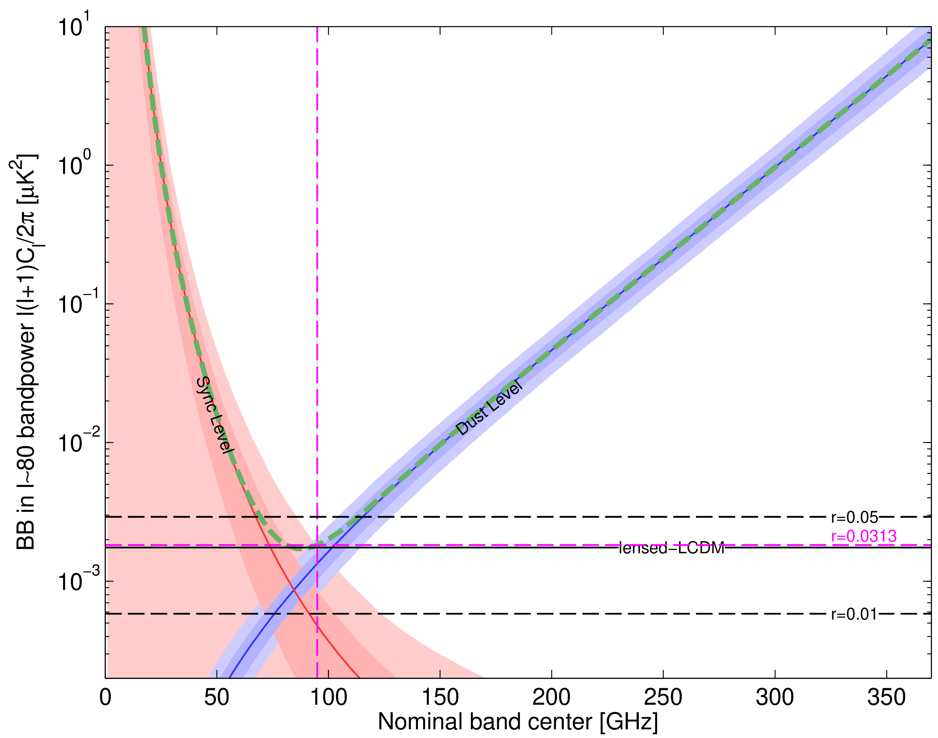
Figure 1 shows the frequency dependence of the foreground amplitudes at the \(\ell \simeq 80\) PGW peak. It is based on the BK15 likelihood results, where we model dust and synchrotron at the cross spectrum level. The shaded regions show the \(1\sigma\) and \(2\sigma\) regions of the synchrotron in red and dust in blue. We also show the mean as solid lines, and the sum in green. We then report the corresponding r at 95GHz, which is really close to the lensed-LCDM level, with \(r\simeq0.0313\).
Figure 1: see BK15 paper, figure 6: Expectation values and noise uncertainties
for the \(\ell\sim80\) BB bandpower in the \biceptwo/\keck\ field.
The solid and dashed black lines show the expected signal power of
lensed-LCDM and \(r_{0.05}=0.05\) \& 0.01.
Since CMB units are used, the levels corresponding
to these are flat with frequency.
The blue/red bands show the 1 and \(2\sigma\) ranges of dust and
synchrotron in the baseline analysis including the uncertainties
in the amplitude and frequency spectral index parameters
(\(A_{s,23 GHz}, \beta_s\) and \(A_{d,353 GHz}, \beta_d\)).
2. Extrapolation to other patches.
If we want to be cautious about potential unmodeled foreground residuals in our maps, we want to somehow estimate how such residual would bias our r-recovery assuming different observed patches.
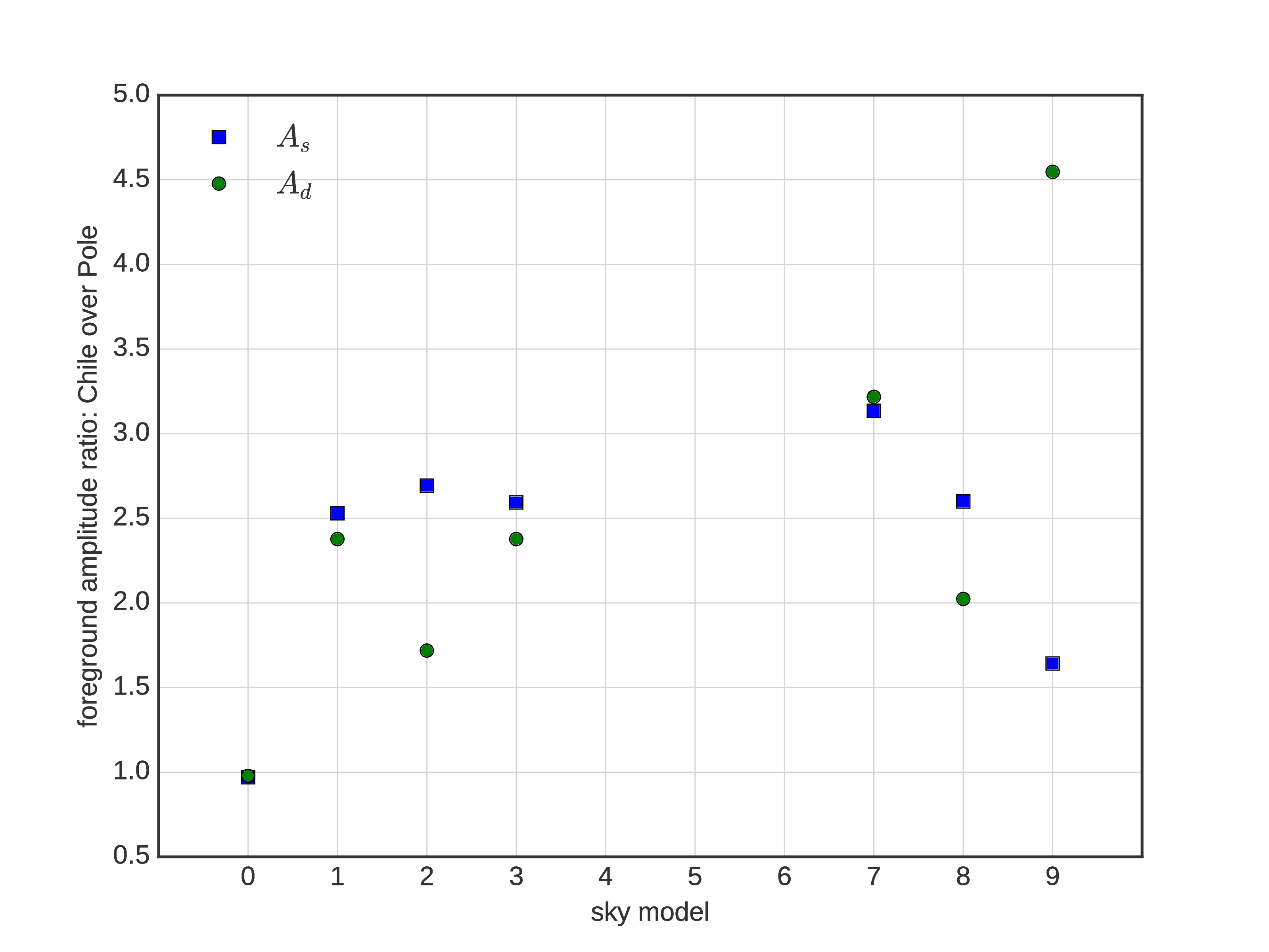
We see in Figure 2 how the foreground amplitude varies between the Pole (B3) and Chile (SO) patches for different simualted sky models.
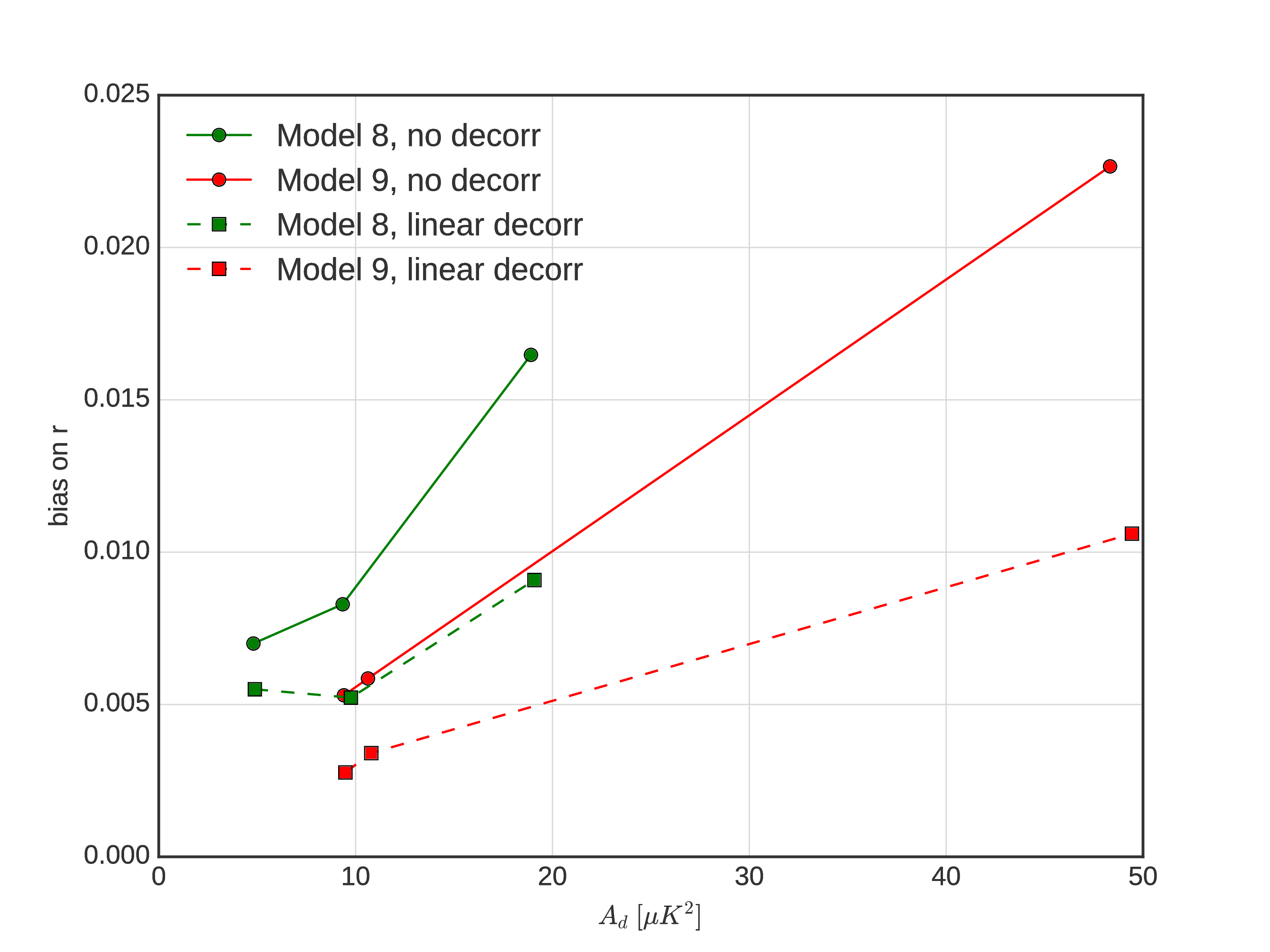
In models that have both data driven variations of the foregrounds on the sky, and enough complexity to produce biases in out recovery of r, we see in Figure 3 that this bias scales roughly linearly with the foreground level.
Comments on figure 2 and 3 (the sky models are described for example in this posting):
Model 0 doesn't have any variation over the sky, as we recover in the ratio.
Models 1, 2, and 3 are PySM models that have variations over the sky constrained by Planck data, but were shown not to reproduce the real sky variations in this posting. Chile seems to have on average 2.5 times more synchrotron. We have similar ratios for dust for model 1 and 3. Model 2 is a bit lower ratio.
Models 4, 5 and 6 haven't been analysed with the Chile and Pole mask (4 and 6 aren't full sky simulations).
Model 7 is a modulated Gaussian model that was based on the amplitude of BB at \(\ell=80\) in planck 353GHz data, to reproduce the variation of foregrounds over the sky. Synchrotron was modulated with the same variations.
Model 8 and 9 also have variations over the sky constrained by data in different ways. Model 8 has multiple layers of varying dust temperature, SED and opticla depth constrained by external data, and it naturally produces decorrelation of the foreground, as well as a flattening of the dust spectra at low frequencies. This in turns will produce biases in our recovered r, since our parametric models assume simpler foregrounds.
Model 9 uses the Planck intensity map at 353GHz and generates polarized maps using multi-layers magnetic fields. It has an adhoc decorrelation modeled by variations of \(\beta_d\) over ths sky based on Planck data. It also produces biases in the recovered r.
Figure 2: Ratio of the foreground level recovered in the ML searches in the Chile patch over the Pole patch, as a function of sky model. We show the results for \(A_d\) in green and \(A_s\) in blue.
Figure 3: Bias on the recovered tensor-to-scalar ratio r as a function of the recovered amplitude of the dust foreground at \(\ell=80\) and 353GHz in \(\mu K^2\). These results were obtained using the the maximum likelihood parametric method for model 8 in green and model 9 in red, for the different masks (DC04, DC04b and DC04c). In these plots, the low-bias low-foreground points are the DC04 (circular mask) whereas the high bias high foregrounds are the Chile masks (DC04b). Solid lines show the results that don't try to fit for decorrelation, whereas the dashed lines are for the case fitting for linear decorrelation.
3. A simple recipe for a mask dependent foreground penalty.
Here, even if we base our Pole value on the BK patch, which is smaller and has probably a lower effective \(A_d\) than the Pole DC04c mask, we can provide a scaling of the foreground residual effects on r recovery for different patches in 2 cases: one where the residuals correspond to 0.5% of the total foreground amplitude, and one where they correspond to 2% of the total foreground amplitude.
Since model 7 is the one that is the most directly related to our current knowledge of variations of the dust B modes amplitude over the sky, we will use this factor of 3.22 between Chile and Pole regions.
Model 7 doesn't have any foreground complexity other that a variation of the amplitude, so to estimate the scaling of the bias on r with foreground amplitude, we will use model 8 and 9. In Figure 3 we see that the slope depends on the model and if we take into account decorrelation or not. In our simple modeling, we will assume that the bias scales directly with the foreground amplitude.
Table 1
Equivalent r from unmodeled foreground residual power at 95GHz for a 0.5% and a 2% residual scenarii. The Pole value is estimated from the measured BK dust power extrapolated at 95GHz, at \(\ell \simeq 80\), the scaling is from a data-constrained sky model with realistic foreground amplitude variations. We assume the scaling of the r-bias to be directly proportional to this scaling.