\(\sigma_r\) forecasting checkpoints, V2

2016-05-31 (Victor Buza)

This posting is a direct update on this posting. For self-containment, I preserve a lot of the text from that posting, with additional text on the updates where necessary. The list of updates is as follows:

Added "no delensing" case to all six checkpoints
Added entry stating the level of residual lensing power for each of the six checkpoints. On this point, also added note (and plot) stating more clearly what assumptions are made for delensing.
Added forecasting results from a Knox implimentation that uses the \(0^{th}\) order information in the tables below. This should make the effect of switching from using simple map-depths and sky area to \(N_l\)'s and fully descriptive BPCM's quite clear. It should also be closer to what other groups have implemented so far.
Made clear note stating that the map-depth numbers are for (Q or U, E or B) polarization maps.
Updated \(N_l\) files with a better header, and added files with interpolated \(N_l\)'s to \(\Delta{l}=1\) spacing, at Jo's request.

The entries in Table 2 and 3 have remained unchanged. Just like in the previous version, I prescribe six \(r\) forecasting checkpoints, and use the machinery described in detail in this posting to arrive at a \(\sigma_r\). These six cases that have been agreed upon are for an effective effort of \(1,000,000\) det-yrs (150 equivalent) on the small-patch part of the S4 survey, for \(f_{sky}=[0.01, 0.05, 0.10]\) and \(r=[0, 0.01]\); to understand what the (150 equivalent) stands for, please see bullet point three in section two of the posting linked above. I should note that these checkpoints are exactly that, and do not necessarily represent the final word on the configuration of S4. Further iterations are certainly within scope. The case definitions are guided by the full optimization and its caveats, described in the posting above, and are grounded in achieved performances (and scalings thereof). As noted in the bullet list above, I have also implemented a Knox BPCM calculation, and included forecasts derived from that as well.

1. Experiment Specification

The three tables below should contain all the information necessary for any forecasting machinery to be able to arrive at a corresponding \(\sigma_r\). The cyan colored boxes represent the \(0^{th}\) order information for a first-pass forecast. In addition, for a more detailed approach, full bandpower window functions, bandpasses, and \(N_l\)'s have also been provided.

Table 1:

This table offers some case-independent experiment specifications. For each of the eight channels considered, there is a center frequency, a \(\Delta\nu/\nu\) for a simple bandpass prescription, a beamwidth, a fully detailed bandpass (caculated using a Chebyshev poly-filtering), and a BPWF prescription.

\(\nu\),GHz	\(\Delta \nu/\nu\)	FWHM, arcmin	Bandpass, [\(\nu\),\(B_{\nu}\)]	BPWF
30	0.30	76.6	bandpass30.txt	bpwfS4.dat
40	0.30	57.5	bandpass40.txt	↑
85	0.24	27.0	bandpass85.txt	\|
95	0.24	24.2	bandpass95.txt	\|
145	0.22	15.9	bandpass145.txt	\|
155	0.22	14.8	bandpass155.txt	\|
215	0.22	10.7	bandpass215.txt	\|
270	0.18	8.5	bandpass270.txt	\|

As mentioned in the text above, the effort distributions in the tables below were calculated given an optimized solution for a minimal \(\sigma_r\), taking into account contributions from foregrounds and CMB lensing. The assumed unit of effort is equivalent to 500 det-yrs at 150 GHz. For other channels, the number of detectors is calculated as \(n_{det,150}\times \left(\frac{\nu}{150}\right)^2\), i.e. assuming comparable focal plane area. A conversion between the (150 equivalent) number of det-yrs and (actual) number of det-yrs is given for each band. This is just one way to implement a detector cost-function, and other suggestions are welcomed.

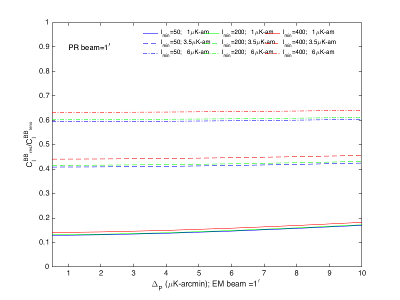
For each case, I list the fraction of effort spent towards solving the foreground separation problem ("degree-scale effort") and reducing the lensing contribution ("arcmin-scale effort"). For the arcminute scale effort, to calculate an effective level of residual lensing, an experiment with \(1\) \(arcmin\) resolution, and mapping speed equivalent to the 145 channel was assumed, hence the conversion between (150 equiv) and (actual); however, all that is necessary to take away (on the delensing front) from these tables are the arcmin-scale map-depths. Then, using an iterative estimator, a \(C_{\ell, res}/C_{\ell, lens}\) is calculated, the results of which are presented in this plot. PR stands for the experiment used for "phi/lensing reconstruction," and EM stands for the experiment (or combination of experiments) used for getting the E-modes. The combined map-depth of EM is assumed to be \(1 \mu K\)-arcmin, though we've seen before (from Kimmy) that the ratio of \(C_{\ell, res}/C_{\ell, lens}\) depends quite little on this noise, as seen here. The \(l_{min}\) in the plot is for the E/B inputs to \(\Phi\); all cases assume complete E-mode coverage (i.e. good coverage for \(l>30\)) for the formation of the B-mode template. Practically, this is a scenario in which the arcmin-scale experiment may be noisy at low \(l\), but we can nonetheless measure all of the E-modes through this range to the level of precision required either with the arcmin-scale or degree-scale experiments. This complete E-mode map is then used to form a B-template by lensing these E-modes with the reconstructed \(\Phi\).

For the various cases, given a fixed effort, the map-depths and \(N_l\)'s are scaled accordingly with \(f_{sky}\).

Table 2:

Case: \(r=0\), Total effort: \(10^6\) det-yrs (150 equiv)

Note: Given the assumed level of foreground complexity, the fully optimal solution presented in this posting does not necessarily divide effort among all of the eight bands. To combat this, an equal force split among bands in each atmospheric window has been implemented. You will notice an equal amount of 150 equiv det-yrs being assigned to each of the two bands in each of the atmospheric windows. Furthermore, as one increases \(f_{sky}\), the optimization algorithm allocates more resources towards the foreground separation problem, and results in some bands "kicking in" after the total \(10^6\) det-yrs threshold. In particular the 145/155 bands for the \(f_{sky}=[0.05, 0.10]\) cases are significantly underused in the optimal solution. To combat this, some effort from the 85/95 channels has been reallocated towards the 145/155 channels. Both of these effects introduce deviations from the optimal solution which are discussed in the posting linked above. All map-depths are quoted for (Q or U, E or B) polarization.

Update: The table has been updated to quote effective residual \(A_L\) for each of the arcmin-scale efforts (in units of power). Also, in addition to the \(N_l\) files with binned values, I added \(N_l\) files that interpolate from the binned values to \(\Delta{l}=1\) spacing.

	\(f_{sky}=0.01\)				\(f_{sky}=0.05\)				\(f_{sky}=0.10\)
\(\nu\),GHz	# det-yrs (150 equiv)	# det-yrs (actual)	map depth, \(\mu K\)-arcmin	\(N_l\), \(\mu K_{CMB}^2\)	# det-yrs (150 equiv)	# det-yrs (actual)	map depth, \(\mu K\)-arcmin	\(N_l\), \(\mu K_{CMB}^2\)	# det-yrs (150 equiv)	# det-yrs (actual)	map depth, \(\mu K\)-arcmin	\(N_l\), \(\mu K_{CMB}^2\)
30	16,250	650	5.62	Nl_r0_fsky1	28,750	1,150	9.46	Nl_r0_fsky5	28,750	1,150	13.37	Nl_r0_fsky10
40	16,250	1,160	5.73	Nl_dl1_r0_fsky1	28,750	2,040	9.64	Nl_dl1_r0_fsky5	28,750	2,040	13.63	Nl_dl1_r0_fsky10
85	127,500	40,940	0.96	↑	170,000	54,590	1.86	↑	186,250	59,810	2.52	↑
95	127,500	51,140	0.79	↑	170,000	68,190	1.53	↑	186,250	74,710	2.06	↑
145	87,500	81,760	0.84	↑	87,500	81,760	1.87	↑	87,500	81,760	2.65	↑
155	87,500	93,430	0.87	↑	87,500	93,430	1.94	↑	87,500	93,430	2.74	↑
215	55,000	112,990	2.14	↑	42,500	87,310	5.43	↑	55,000	112,990	6.76	↑
270	55,000	178,200	3.20	↑	42,500	137,700	8.14	↑	55,000	178,200	10.11	↑
Total Degree Scale Effort	572,500	560,270	~	~	657,500	526,180	~	~	715,000	604,100	~	~
Total Arcmin Scale Effort	427,500	399,470	0.38 (A_L=0.048)	~	342,500	320,050	0.94 (A_L=0.121)	~	285,000	266,320	1.47 (A_L=0.188)	~
Total Effort	1,000,000	959,740	~	~	1,000,000	846,230	~	~	1,000,000	870,420	~	~

Table 3:

Case: \(r=0.01\), Total effort: \(10^6\) det-yrs (150 equiv)

Note: See Note from Table 2.

Update: The table has been updated to quote effective residual \(A_L\) for each of the arcmin-scale efforts (in units of power). Also, in addition to the \(N_l\) files with binned values, I added \(N_l\) files that interpolate from the binned values to \(\Delta{l}=1\) spacing.

	\(f_{sky}=0.01\)				\(f_{sky}=0.05\)				\(f_{sky}=0.10\)
\(\nu\),GHz	# det-yrs (150 equiv)	# det-yrs (actual)	map depth, \(\mu K\)-arcmin	\(N_l\), \(\mu K_{CMB}^2\)	# det-yrs (150 equiv)	# det-yrs (actual)	map depth, \(\mu K\)-arcmin	\(N_l\), \(\mu K_{CMB}^2\)	# det-yrs (150 equiv)	# det-yrs (actual)	map depth, \(\mu K\)-arcmin	\(N_l\), \(\mu K_{CMB}^2\)
30	28,750	1,150	4.23	Nl_r01_fsky1	41,250	1,650	7.89	Nl_r01_fsky5	41,250	1,650	11.16	Nl_r01_fsky10
40	28,750	2,040	4.31	Nl_dl1_r01_fsky1	41,250	2,930	8.04	Nl_dl1_r01_fsky5	41,250	2,930	11.38	Nl_dl1_r01_fsky10
85	151,250	48,570	0.88	↑	195,000	62,620	1.74	↑	211,250	67,830	2.36	↑
95	151,250	60,670	0.72	↑	195,000	78,220	1.43	↑	211,250	84,730	1.94	↑
145	50,000	46,720	1.11	↑	50,000	46,720	2.48	↑	50,000	46,720	3.50	↑
155	50,000	53,390	1.45	↑	50,000	53,390	2.56	↑	50,000	53,390	3.62	↑
215	42,500	87,310	2.43	↑	42,500	87,310	5.44	↑	42,500	87,310	7.69	↑
270	42,500	137,700	3.64	↑	42,500	137,700	8.13	↑	42,500	137,700	11.50	↑
Total Degree Scale Effort	545,000	437,550	~	~	657,500	470,540	~	~	690,000	482,280	~	~
Total Arcmin Scale Effort	455,000	425,170	0.37 (A_L=0.047)	~	342,500	320,050	0.95 (A_L=0.122)	~	310,000	289,680	1.41 (A_L=0.181)	~
Total Effort	1,000,000	862,720	~	~	1,000,000	790,590	~	~	1,000,000	771,960	~	~

2. Worked-out implementation using our full framework; parameter constraints and \(\sigma_r\) performance

In this section, I use fully descriptive BPCM's (more details about the treatment of noise and signal in the formation of the BPCM can be found in Section 1 of this posting) as inputs to the Fisher Forecasting framework (described in Sections 1 and 2 of the same posting linked above). However, the \(N_l\) files above should be compatible with the used BPCM's.

The Fisher matrix I'm considering is 8-dimensional. The 8 parameters we are constraining are: {\(r, A_{dust}, \beta_{dust}, \alpha_{dust}, A_{sync}, \beta_{sync}, \alpha_{sync}, \epsilon\)}. Where \(\beta_{dust}\) and \(\beta_{sync}\) have Gaussian priors of \(0.11, 0.30\), and the rest have flat priors. For a more detailed description of the parameters used in the model, see the "Multicomponent Model" subsection in Section 1 of the posting linked above.

The Fiducial Model for the Fisher forecasting is centered at either \(r\) of 0 or 0.01, with \(A_{dust,l=80}^{\nu=353} = 4.25\) (best-fit value from BK14) and \(A_{sync, l=80}^{\nu=23}=3.8\) (95% upper limit from BK14). The spatial and frequency spectral indeces are centered at \(\beta_{dust}=1.59, \beta_{sync}=-3.10, \alpha_{dust}=-0.42, \alpha_{sync}=-0.6\), and the dust/sync correlation is centered at \(\epsilon=0\).

For an illustration of the full dimensionality and the degeneracies of the Fisher matrix being constrained in this implementation, see this Fisher ellipse plot for the \(r=0\), \(f_{sky}=0.01\) case.

As one scales \(f_{sky}\) up, there are of course a number of caveats to keep in mind for this implimentation, all of which are described in a bullet-point list in the preamble to Figure 3 of this posting.

Table 4:

For each of the six cases decribed above, I marginalize over the fully dimensional Fisher Matrix to arrive at the following \(\sigma_r\) results. The \(A_L<1\) nomenclature stands for -- delensing included at the levels specified in Tables 2 and 3, and the \(A_L=1\) stands for -- no-delensing included.

	\(f_{sky}=0.01\)	\(f_{sky}=0.05\)	\(f_{sky}=0.10\)
\(\sigma_r(r=0, A_L<1), \times 10^{-3}\)	0.55	0.81	0.95
\(\sigma_r(r=0, A_L=1), \times 10^{-3}\)	6.14	3.09	2.44
\(\sigma_r(r=0.01, A_L<1), \times 10^{-3}\)	1.85	1.44	1.42
\(\sigma_r(r=0.01, A_L=1), \times 10^{-3}\)	7.92	3.85	2.98

It is worth noting that this framework has been validated against simulations at the BKP and BK14 noise-levels, and further development is in progress to perform validations with map-level simulations of skies with various degrees of complexity, provided by groups such as Jo/Ben/David or Ghosh/Aumont/Boulanger.

3. Knox implementation; \(\sigma_r\) performance

In addition to the constraints above which have been derived with the full machinery, and using scalings from achieved surveys, I have implemented a version that relies on a Knox equivalent formulation of the BPCM that uses the \(0^{th}\) order information in the tables above. The Knox equivalent formulation uses top-hat bandpower window functions, centered at the nominal values of the 9 BICEP/Keck bins, each with a width of \(\Delta{l}=35\). The foreground expectation values are derived using the same multicomponent modelling and fiducial model as in the section above. The resulting constraints are presented in the table below.

Table 5:

\(\sigma_r\) constraints derived from a Knox equivalent formulation of the BPCM. For each of the six cases decribed above, I marginalize over the fully dimensional Fisher Matrix to arrive at the following \(\sigma_r\) results. The \(A_L<1\) nomenclature stands for -- delensing included at the levels specified in Tables 2 and 3, and the \(A_L=1\) stands for -- no-delensing included.

	\(f_{sky}=0.01\)	\(f_{sky}=0.05\)	\(f_{sky}=0.10\)
\(\sigma_r(r=0, A_L<1), \times 10^{-3}\)	0.23	0.31	0.36
\(\sigma_r(r=0, A_L=1), \times 10^{-3}\)	3.59	1.70	1.27
\(\sigma_r(r=0.01, A_L<1), \times 10^{-3}\)	1.30	0.87	0.77
\(\sigma_r(r=0.01, A_L=1), \times 10^{-3}\)	5.02	2.33	1.72

Comparing Table 4 and Table 5, one sees a clear difference in the achieved constraints.In particular, as expected, Table 5 has more optimistic numbers. Below I list a number of effects that are included in the full treatment described in Section 2, and previous postings, and not included in Section 3, which should explain the weaker constraints of Section 2. Section 2 uses/includes:

A fully descrpitive BPCM, including \(l\)-bin correlations.
Realistic \(N_l\)'s that include excss low ell noise vs simple white noise \(N_l\)'s. Given that most of the component separation happens at degree scales, this is potentially a significant factor.
Mode filtering which affect sky coverage and S/N per mode.
Noise contributions to BPCM that take into account the non-uniformity of our surveys; these result in effectively wider/shallower maps than Knox which assumes a uniform distribution of survey-weight over a given \(f_{sky}\).

Note about comparisons to other groups: Since the inception of this posting, Stephen and Josquin have updated their posting. Since they use the \(0^{th}\) order information, their numbers should be compared to the ones in my Table 5. In doing so, one can extract the following numbers from their posting, which I put in a format similar to above:

Table 6:

The second row is taken from the no-delensing case they have in their second table of their Section 1. The first row is taken from their 31/05/2016 update that has \(l_{min}=30\) for their B-template and reconstructed \(\Phi\), which I believe to be the closest to our delensing implementation (though this needs to be confirmed).

	\(f_{sky}=0.01\)	\(f_{sky}=0.05\)	\(f_{sky}=0.10\)
\(\sigma_r(r=0, A_L<1), \times 10^{-3}\)	0.22	0.31	0.36
\(\sigma_r(r=0, A_L=1), \times 10^{-3}\)	3.44	1.65	1.23

It is clear that there is fairly good agreement for these two scenarios. While the agreement for the no-delensing case does not necessarily mean that the two component separation methods are equally powerful (since both sample variance limited on lensing in this case; though it is reassuring that they're seeing similar level of lensing sample variance), the agreement for the delensing-included case perhaps hints to the fact that these two different methods achieve comparable component separation in this limit.

Concluding Notes:

The fact that the effects listed below Table 5 degrade our constraints shouldn't really come as a surprise, and is precisely the reason we believe that forecasting should be grounded in achieved perfomances. It is possible that we might do better on some of these points with a different survey design, and in that case, perhaps the numbers in Tables 4 and 5 bracket the list of possible outcomes. I should also note that for the purposes of comparisons to other groups, I have turned off effects such as dust decorrelation, which we've seen in this posting degrades the contraints by tens of percent. If turning these effects (and other realistic penalties for systematics and variable foregrounds, that have not yet been included in these forecasts) would then mean that we are not able to achieve the desired \(\sigma_r\) required for the S4 science goals, then we are perhaps in a scenario in which the science drivers dictate the survey definition, and we could boost the total effort from \(10^6\) det-yrs (150 equiv) to some larger amount.