\(\sigma_r\) forecasting checkpoints

In this posting I prescribe six reference cases for \(r\) forecasting, and use the machinery described in detail in this posting to arrive at a \(\sigma_r\). These six cases that have been agreed upon are for an effective effort of \(1,000,000\) det-yrs (150 equivalent) on the small-patch part of the S4 survey, for \(f_{sky}=[0.01, 0.05, 0.10]\) and \(r=[0, 0.01]\); to understand what the (150 equivalent) stands for, please see bullet point three in section two of the posting linked above. The case definitions are guided by the full optimization and its caveats, described in the posting above, and are grounded in achieved performances (and scalings thereof).

1. Experiment Specification

The three tables below should contain all the information necessary for any forecasting machinery to be able to arrive at a corresponding \(\sigma_r\). The cyan colored boxes represent the \(0^{th}\) order information for a first-pass forecast. In addition, for a more detailed approach, full bandpower window functions, bandpasses, and \(N_l\)'s have also been provided.

Table 1:

This table offers some case-independent experiment specifications. For each of the eight channels considered, there is a center frequency, a \(\Delta\nu/\nu\) for a simple bandpass prescription, a beamwidth, a fully detailed bandpass (caculated using a Chebyshev poly-filtering), and a BPWF prescription.

\(\nu\),GHz	\(\Delta \nu/\nu\)	FWHM, arcmin	Bandpass, [\(\nu\),\(B_{\nu}\)]	BPWF
30	0.30	76.6	bandpass30.txt	bpwfS4.dat
40	0.30	57.5	bandpass40.txt	↑
85	0.24	27.0	bandpass85.txt	\|
95	0.24	24.2	bandpass95.txt	\|
145	0.22	15.9	bandpass145.txt	\|
155	0.22	14.8	bandpass155.txt	\|
215	0.22	10.7	bandpass215.txt	\|
270	0.18	8.5	bandpass270.txt	\|

As mentioned in the text above, the effort distributions in the tables below were calculated given an optimized solution for a minimal \(\sigma_r\), taking into account contributions from foregrounds and CMB lensing. The assumed unit of effort is equivalent to 500 det-yrs at 150 GHz. For other channels, the number of detectors is calculated as \(n_{det,150}\times \left(\frac{\nu}{150}\right)^2\), i.e. assuming comparable focal plane area. A conversion between the (150 equivalent) number of det-yrs and (actual) number of det-yrs is given for each band. This is just one way to implement a detector cost-function, and other suggestions are welcomed.

For each case, I list the fraction of effort spent towards solving the foreground separation problem ("degree-scale effort") and reducing the lensing contribution ("arcmin-scale effort"). For the arcminute scale effort, to calculate an effective level of residual lensing, an experiment with \(1\) \(arcmin\) resolution, and mapping speed equivalent to the 145 channel was assumed, hence the conversion between (150 equiv) and (actual); however, all that is necessary to take away (on the delensing front) from these tables are the arcmin-scale map-depths.

For the various cases, given a fixed effort, the map-depths and \(N_l\)'s are scaled accordingly with \(f_{sky}\).

Table 2:

Case: \(r=0\), Total effort: \(10^6\) det-yrs (150 equiv)

Note: Given the assumed level of foreground complexity, the fully optimal solution presented in the previous posting does not necessarily divide effort among all of the eight bands. To combat this, an equal force split among bands in each atmospheric window has been implemented. You will notice an equal amount of 150 equiv det-yrs being assigned to each of the two bands in each of the atmospheric windows. Furthermore, as one increases \(f_{sky}\), the optimization algorithm allocates more resources towards the foreground separation problem, and results in some bands "kicking in" after the total \(10^6\) det-yrs threshold. In particular the 145/155 bands for the \(f_{sky}=[0.05, 0.10]\) cases are significantly underused in the optimal solution. To combat this, some effort from the 85/95 channels has been reallocated towards the 145/155 channels. Both of these effects introduce deviations from the optimal solution which are discussed in the posting linked above.

	\(f_{sky}=0.01\)				\(f_{sky}=0.05\)				\(f_{sky}=0.10\)
\(\nu\),GHz	# det-yrs (150 equiv)	# det-yrs (actual)	map depth, \(\mu K\)-arcmin	\(N_l\), \(\mu K_{CMB}^2\)	# det-yrs (150 equiv)	# det-yrs (actual)	map depth, \(\mu K\)-arcmin	\(N_l\), \(\mu K_{CMB}^2\)	# det-yrs (150 equiv)	# det-yrs (actual)	map depth, \(\mu K\)-arcmin	\(N_l\), \(\mu K_{CMB}^2\)
30	16,250	650	5.62	Nl_r0_fsky1	28,750	1,150	9.46	Nl_r0_fsky5	28,750	1,150	13.37	Nl_r0_fsky10
40	16,250	1,160	5.73	↑	28,750	2,040	9.64	↑	28,750	2,040	13.63	↑
85	127,500	40,940	0.96	↑	170,000	54,590	1.86	↑	186,250	59,810	2.52	↑
95	127,500	51,140	0.79	↑	170,000	68,190	1.53	↑	186,250	74,710	2.06	↑
145	87,500	81,760	0.84	↑	87,500	81,760	1.87	↑	87,500	81,760	2.65	↑
155	87,500	93,430	0.87	↑	87,500	93,430	1.94	↑	87,500	93,430	2.74	↑
215	55,000	112,990	2.14	↑	42,500	87,310	5.43	↑	55,000	112,990	6.76	↑
270	55,000	178,200	3.20	↑	42,500	137,700	8.14	↑	55,000	178,200	10.11	↑
Total Degree Scale Effort	572,500	560,270	~	~	657,500	526,180	~	~	715,000	604,100	~	~
Total Arcmin Scale Effort	427,500	399,470	0.38	~	342,500	320,050	0.94	~	285,000	266,320	1.47	~
Total Effort	1,000,000	959,740	~	~	1,000,000	846,230	~	~	1,000,000	870,420	~	~

Table 3:

Case: \(r=0.01\), Total effort: \(10^6\) det-yrs (150 equiv)

Note: See Note from Table 2.

	\(f_{sky}=0.01\)				\(f_{sky}=0.05\)				\(f_{sky}=0.10\)
\(\nu\),GHz	# det-yrs (150 equiv)	# det-yrs (actual)	map depth, \(\mu K\)-arcmin	\(N_l\), \(\mu K_{CMB}^2\)	# det-yrs (150 equiv)	# det-yrs (actual)	map depth, \(\mu K\)-arcmin	\(N_l\), \(\mu K_{CMB}^2\)	# det-yrs (150 equiv)	# det-yrs (actual)	map depth, \(\mu K\)-arcmin	\(N_l\), \(\mu K_{CMB}^2\)
30	28,750	1,150	4.23	Nl_r01_fsky1	41,250	1,650	7.89	Nl_r01_fsky5	41,250	1,650	11.16	Nl_r01_fsky10
40	28,750	2,040	4.31	↑	41,250	2,930	8.04	↑	41,250	2,930	11.38	↑
85	151,250	48,570	0.88	↑	195,000	62,620	1.74	↑	211,250	67,830	2.36	↑
95	151,250	60,670	0.72	↑	195,000	78,220	1.43	↑	211,250	84,730	1.94	↑
145	50,000	46,720	1.11	↑	50,000	46,720	2.48	↑	50,000	46,720	3.50	↑
155	50,000	53,390	1.45	↑	50,000	53,390	2.56	↑	50,000	53,390	3.62	↑
215	42,500	87,310	2.43	↑	42,500	87,310	5.44	↑	42,500	87,310	7.69	↑
270	42,500	137,700	3.64	↑	42,500	137,700	8.13	↑	42,500	137,700	11.50	↑
Total Degree Scale Effort	545,000	437,550	~	~	657,500	470,540	~	~	690,000	482,280	~	~
Total Arcmin Scale Effort	455,000	425,170	0.37	~	342,500	320,050	0.95	~	310,000	289,680	1.41	~
Total Effort	1,000,000	862,720	~	~	1,000,000	790,590	~	~	1,000,000	771,960	~	~

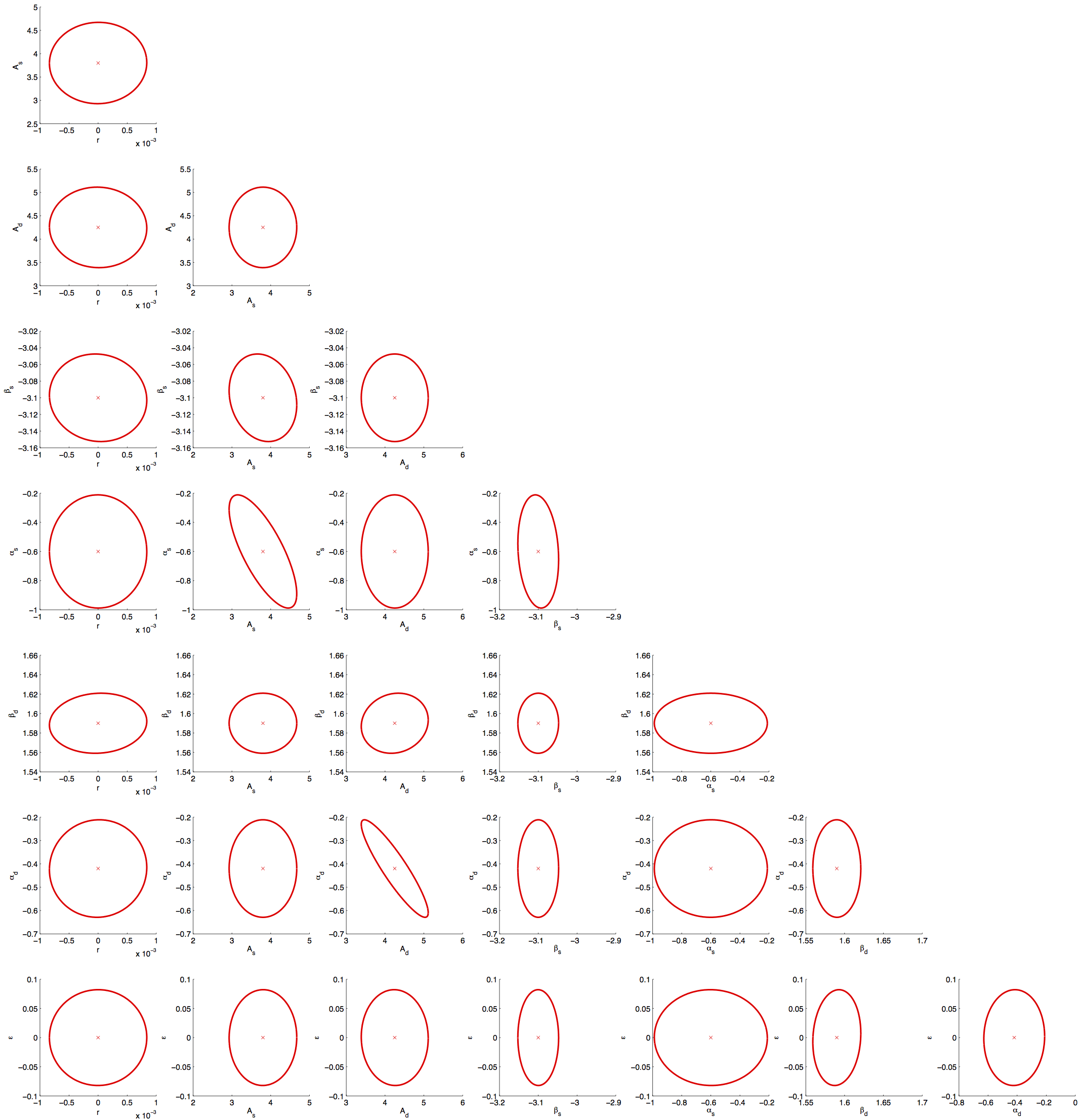
2. Worked-out implementation; parameter constraints and \(\sigma_r\) performance

In this section, I use fully descriptive BPCM's (more details about the treatment of noise and signal in the formation of the BPCM can be found in Section 1 of this posting) as inputs to the Fisher Forecasting framework (described in Sections 1 and 2 of the same posting linked above). However, the \(N_l\) files above should be compatible with the used BPCM's.

Table 4:

For each of the six cases decribed above, I marginalize over the fully dimensional Fisher Matrix to arrive at the following \(\sigma_r\) results.

	\(f_{sky}=0.01\)	\(f_{sky}=0.05\)	\(f_{sky}=0.10\)
\(\sigma_r(r=0), \times 10^{-4}\)	5.52	8.06	9.51
\(\sigma_r(r=0.01), \times 10^{-3}\)	1.85	1.44	1.42

It is worth noting that this framework has been validated against simulations at the BKP and BK14 noise-levels, and further development is in progress to perform validations with map-level simulations of skies with various degrees of complexity, provided by groups such as Jo/Ben/David or Ghosh/Aumont/Boulanger.