Inspecting DM reference design sims

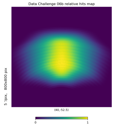
2020-08-17 (C. Bischoff)
UPDATE 2020-08-20: Finished figure captions and explanatory text

This posting repeats and extends the analysis from my 2020-05-19 posting. A new iteration of the reference design sims has been generated that was meant to fix the discrepancies in white noise levels seen in that previous round. In the process of working through this verification, we discovered that the CIB simulations had large spurious polarization, which has now been fixed. The plots below provide a brief summary of the signal and noise components of the sims.

Hits maps

The hits maps are unchanged from my previous posting. Compared to Data Challenge 06b from the Low-ℓ BB analysis working group, these sims has somewhat narrower coverage at 30–155 GHz and somewhat broader coverage at 220/270 GHz. The reason for this difference is that these sims include a high-frequency (220/270) SAT with smaller aperture size and larger field of view.

Figure 1:

Relative hit maps for Data Challenge 06b sims (left) and DM sims (right). Note that the DC 06b sims use the same hit map for all frequencies, while the hit map for the DM sims varies with frequency.

All power spectra in the subsequent sections are obtained by weighting by the hits maps (equivalent to inverse noise variance weighting) and then running healpy.anafast. I correct the resulting power spectra for the weighting mask area, but no attempt is made to correct for mixing of power in ℓ or mixing between E and B. Instead, I have focused on spectra where E→B leakage won't significantly affect the conclusions, i.e. using EE spectrum from CMB maps and EE+BB spectra for foreground and noise maps that don't feature large E/B asymmetry.

Suppression factor

The DM sims have signal suppression due to time-domain filtering. To get an estimate of this effect, I calculated the EE spectrum of the CMB-only maps and took the ratio against an EE theory spectrum multiplied by Gaussian \(\mathcal{B}_\ell^2\). The orange line is an attempt to fit the curve with a simple functional form:

\[ \begin{equation} f(\ell) = \left\{ \begin{array}{ll} 0 \, , & \ell \le 20 \\ 1 - \exp \left[ (\ell - 20) / \ell_0 \right] \, , & \ell \gt 20 \end{array} \right. \end{equation} \]

Recall that we have only one CMB realization, so the suppression factor estimate is very noisy! The values that I obtain for \(\ell_0\) range from 91 (at 270 GHz) to 107 (at 30 GHz). The purpose of obtaining this estimate is so that I can correct the low-ℓ power in my analysis of foreground and noise maps below.

For 30/40 GHz, this calculation goes crazy for \(\ell \gt 350\). The beam suppression is very large at these frequencies, so we are taking the ratio of two very small numbers. The EE theory spectrum and \(\mathcal{B}_\ell^2\) can be calculated just fine, but the EE spectrum obtained from the CMB maps has extra power at high \(\ell\) due to the apodization mask, so the spectrum doesn't follow the expectation. This should not cause any issues in practice because we won't be using \(\ell \gt 350\) data from a telescope with 72 arcmin beam.

Figure 2:

Estimate of signal suppression in EE/BB power spectra, obtained by taking the ratio of the measured and theory EE spectra (blue line). The orange curve is a fit using the model shown in Equation 1 above.

Foreground power spectra

Next, I calculated the power spectra of the foreground maps. These maps use PySM model-0 for dust, synchrotron, free-free, and AME, plus CIB, KSZ, and TSZ from WebSky, as documented here. For polarization measurements, only dust and synchrotron are important (once we fixed the CIB bug that was described in the introduction).

In the pager, the dark red line is the power spectrum of the foreground sim maps; the lighter red line has been corrected for the analytic fit to the suppression factor (EE and BB only). The dashed black line shows the Gaussian foreground model used in the Low-ℓ BB Data Challenges—this has \(A_\mathrm{dust} = 4.25\) \(\mu K^2\) (at 353 GHz and ℓ=80) and \(A_\mathrm{sync} = 3.8\) \(\mu K^2\) (at 23 GHz and ℓ=80). The DM sims seem to have a very similar level of polarized synchrotron, but the polarized dust is much brighter than our Gaussian model. In past Low-ℓ BB Data Challenges, we have seen that most PySM models have much brighter dust than is seen by BICEP/Keck.

Figure 3:

Power spectra of foreground maps, in the form of \(\mathcal{D}_\ell\). Dark red is the raw spectrum; light red has been corrected by the model fit to the suppression factor from the previous section (assuming the same suppression factor for EE and BB). The dashed black line corresponds to the Gaussian foreground model used in Low-ℓ BB data challenges. Spectra shown here have *not* been corrected for power suppression due to beam smoothing.

Noise power spectra

Figure 4 compares the noise power spectra between the DM sims and Low-ℓ BB DC 06b. The grey lines are five realizations of 06b. The red lines are noise spectra for the DM sims with (light red) or without (dark red) the suppression factor correction. Note that these spectra are \(\mathcal{C}_\ell\), not \(\mathcal{D}_\ell\), and have not been corrected for beam suppression, so flat lines correspond to white noise.

Overall, the agreement is quite a bit better than in the previous posting. The DM sims now feature some excess low-ℓ polarization noise, which is implemented via leakage of atmospheric noise. However, there are still several questions to investigate:

The DM sims generally have lower white noise than the what was forecast in the DSR. This is especially pronounced at the four highest frequencies, but those four frequencies also show non-white noise out to ℓ∼500 and above. One possible explanation is that the DM sims are using an optimistic assumption for observing efficiency but also have more atmospheric noise leaking into polarization with a red spectrum.

After suppression factor correction, the DM sims predict a bit more low-ℓ excess noise that the Low-ℓ BB sims, which copy the shape of the BICEP/Keck \(\mathcal{N}_\ell\) curves.

In TT we still see very large discrepancy (∼2 orders of magnitude in power!) in noise power between the DM sims and scaled BICEP/Keck performance. The disagreement is much smaller at 30 and 40 GHz.

Given the role of simulated atmospheric noise in the low-ℓ polarization noise for the DM sims, it seems fairly important to understand the huge discrepancy in temperature noise. An obvious action item, which has been in limbo for months, is for Colin to pass some Keck Array timestream data to Reijo, so that he can conduct his noise analysis and compare to similar results from SPT data.

Figure 4:

Power spectra of noise maps, in the form of \(\mathcal{C}_\ell\). The dark red line is the raw noise spectrum from the DM sims; light red has been corrected for the model fit to the filter suppression, as described above. Gray line show the noise spectra for five realizations of the Low-ℓ BB DC 06b sims. Dashed black lines correspond to the white noise level from Table 2-1 of the DSR. Spectra shown here have *not* been corrected for signal suppression due to beam smoothing.