Figure 1:
Relative hit maps for Data Challenge 06b sims (left) and Data Management sims (right). Note that the DC 06b sims use the same hit map for all frequencies, while the hit map for the DM sims varies with frequency.
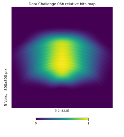
(C. Bischoff)
In this posting, I compare simulations produced by s4_design_sim_tool (which I will refer to as the “DM sims”) to the Data Challenge 06b simulations produced in the Low-ℓ BB analysis working group (“Low-ℓ BB sims”). Both sets of simulations are meant to follow the DSR instrument configuration for the SATs and a Pole-deep survey strategy.
Code used for analysis and figures in this posting: check_sim_noise.py
First, we can compare the hits maps shown in Figure 1. Both the DM and Low-ℓ BB sims use hits maps made by Reijo, but they do have some differences. The Low-ℓ BB sims use the same hits maps at all frequencies, while the DM sims use one hits map for 30/40 GHz, a second one for 85/145 and 95/155, and a third hits map for 220/270 GHz. The DM 220/270 GHz hits map covers a notably larger sky area, despite the fact that all SATs should have similar field of view. Table 1 lists the effective \(f_\mathrm{sky}\) for each hit map, following equation A.1 of the DSR with weighting equal to the hits map (i.e. inverse noise variance weighting). At frequencies other than 220 and 270 GHz, the DM sims have \(f_\mathrm{sky}\) that is smaller by ∼20%, so we might expect \(\mathcal{N}_\ell\) to be ∼20% lower as well, if the total sensitivities are equal. For 220 and 270 GHz, the DM sims have \(f_\mathrm{sky}\) that is 33% higher.
| Frequency | DC 06b \(f_\mathrm{eff}^\mathrm{noise}\) | DM sim \(f_\mathrm{eff}^\mathrm{noise}\) |
|---|---|---|
| 30 GHz | 2.955% | 2.427% |
| 40 GHz | ||
| 85 GHz | 2.418% | |
| 95 GHz | ||
| 145 GHz | ||
| 155 GHz | ||
| 220 GHz | 3.916% | |
| 270 GHz |
Next, Figure 2 shows the \(\mathcal{N}_\ell\) calculated from these maps, after weighting by the hits map (inverse noise variance weighting). The power spectrum estimator is anafast—no pure-B estimator is needed since the noise power is symmetric between E and B. For EE and BB, the dashed black line indicates the \(\mathcal{N}_\ell\) corresponding to the “Q/U rms” line from DSR Table 2-1. Note that the maps analyzed here were generated after the bug fix described here.
| Frequency | DSR Table 2-1 \(\mathcal{N}_\ell^{BB}\) \([\mu K^2]\) | Low-ℓ BB sim \(\mathcal{N}_\ell^{BB}\) \([\mu K^2]\) | DM sim \(\mathcal{N}_\ell^{BB}\) \([\mu K^2]\) |
|---|---|---|---|
| 30 GHz | 1.04e-06 | 0.97e-06 | 0.63e-06 |
| 40 GHz | 1.71e-06 | 1.55e-06 | 0.67e-06 |
| 85 GHz | 6.55e-08 | 6.16e-08 | 3.65e-08 |
| 95 GHz | 5.15e-08 | 4.75e-08 | 4.78e-08 |
| 145 GHz | 1.22e-07 | 1.26e-07 | 0.28e-07 |
| 155 GHz | 1.43e-07 | 1.44e-07 | 0.55e-08 |
| 220 GHz | 1.04e-06 | 0.95e-06 | 0.53e-06 |
| 270 GHz | 3.05e-06 | 2.81e-06 | 1.62e-06 |
Andrea has produced CMB signal sims (ΛCDM, r=0). I have started looking at these, to understand the filtering that has gone into the DM sim maps and how much this affects our interpretation of the noise. In the process of tracking down the cause of the discrepancies seen above, we should improve and centralize the sim documentation.