Simple 1D model to study the effect of different observation strategies on the bandpower statistics.

In this posting we use a 1D model to test analytic formulas of the statistics of signal and non-uniform noise bandpowers.
We then use this simple model to predict the evolution of these statistics depending on different observation strategies, for example varying the field of view of our telescopes.

1. Inputs

1.1 Hitcount maps

We created different types of hitcount maps in map domain to mimick observations with different field of views (circles with radius from 8 to 18 degrees).
They are based on an observation strategy close to the BK one. BICEP/Keck currently observes the sky at a fixed elevation (centered on 57.5 degrees) for 2*50 minutes and scan in azimuth with a width of 64.2 degrees, of which we keep the central constant speed 56.4 degrees. We step by 0.25 degrees every 2*50 minutes. Between 2 steps, the field moves by 2*50/60*15 = 25 degrees. These steps cover 5 degrees in elevation.
Thus, the telescope roughly points on a rectangle of height 5° and width (56.4°)*cos(57.5°)=30.3°. Due to the sky rotation, there is an additional slightly tapered 25°*cos(57.5°)=13.4°.
Here we approximate this observed patch on a flat sky by a rectangle of width 38 degrees and height 5 degrees, on a full sky of 203°x203°. We then convolve with a circle to simulate the field of view of the instrument. We vary the radius of these circles between 8 and 18 degrees. These different hitmaps are shown in Figure 1.

For the rest of the posting, we will use a toy model in 1D with signal and noise vectors. For the hitcount vectors, we will use the cumulative distributions of these hitmaps, remapped to \(N_{\rm modes}\)=10000 by interpolation, and normalized so that their sum is 1. These 1D hitcounts are shown in Figure 2, compared to the similarily derived hitcount vectors of the DC04, DC04b, DC04c and BK14 hitmaps.
We can note that while BICEP2/Keck is supposed to have a 20° field of view, and BICEP3 has 28°, they appear shallower than our simple model. These are not circular field of view though, more of a square that is rotated every 48 hours. In this figure it seems like our simple model doesn't exactly reproduce the BK or B3 hitcount distribution. This could maybe better approximated by a tapered circular FOV. Here we mostly care about the general dependence on the FOV though.

1.2 Noise

We generate \(N_{\rm sim}\)=10000 vectors \(x_i\), with \(N_{\rm modes}\)=10000 random Gaussian numbers with \(\sigma_n=1\) and \(\mu_n=0\).

We use the hitcount vectors to generate "observed" noise vectors: \begin{align*} n_i=\frac{x_i}{\sqrt{h_i}} \end{align*}
In Figure 3, we show one example of such noise vector for each hitcount case.

1.2 Signal

We generated \(N_{\rm sim}\)=10000 vectors \(s_i\), with \(N_{\rm modes}\)=10000 random Gaussian numbers with \(\sigma_s=0.1\) and \(\mu_s=0\).

2. Analysis

We then want to estimate a single bandpower from a given data vector \(d_i\): \begin{align*} {\rm\widehat{BP}} &= \frac{\sum_i (w_i*d_i)^2}{\sum_i w_i^2 } \end{align*}
We compute the \(N_{sim}\) bandpowers estimates and compute the mean and variance.
We also compute the effective number of degrees of freedom \(k\): \begin{align*} k &= 2 \frac{ \\< {\rm BP}>^2}{{\rm Var(BP)}} \end{align*}
This is related to the "Effective \(f_{\rm sky}\)" of a map, defined as : \begin{align*} f_{\rm sky,eff} &= \frac{k}{N_{\rm modes}} \end{align*}

In figure 4, we compare the MC numerical results (colored points) to a model (grey bars), derived in these notes.
We show the general case here the weights used are different from the hitcount mas, as well as the case where w=h:

• For the noise bandpowers: \begin{align} { \\<{\rm BP}>} &= \sigma_n^2 \frac{\sum_i w_i^2 h_i^{-1}}{\sum_i w_i^{2}} \;\; \stackrel{w=h}{\longrightarrow} \;\; \sigma_n^2 \frac{\sum_i h_i}{\sum_i h_i^{2}} , \end{align} \begin{align} {\rm Var(BP)} &= 2 \sigma_n^4 \frac{\sum_i w_i^4 h_i^{-2}}{\left(\sum_i w_i^{2}\right)^2} \;\; \stackrel{w=h}{\longrightarrow} \;\; 2 \sigma_n^4 \frac{1}{\sum_i h_i^{2}}, \end{align} and \begin{align} {\rm f_{\rm sky,eff}} &= \frac{\\< w_i^2 h_i^{-1} > ^2}{\\< w_i^{4}h_i^{-2}>} \;\; \stackrel{w=h}{\longrightarrow} \;\; \frac{\\< h_i > ^2}{\\< h_i^{2}>}, \end{align}
• For the signal bandpowers, we found: \begin{align} { \\<{\rm BP}>} &= \sigma_s^2 , \end{align} \begin{align} {\rm Var(BP)} &= 2 \sigma_s^4 \frac{ \sum_i w_i^{4} }{\left(\sum_i w_i^{2}\right)^2} \;\; \stackrel{w=h}{\longrightarrow} \;\; 2 \sigma_s^4 \frac{ \sum_i h_i^{4} }{\left(\sum_i h_i^{2}\right)^2} , \end{align} and \begin{align} {\rm f_{\rm sky,eff}} &= \frac{ \\< w_i^2 >^2}{\\< w_i^{4} >} \;\; \stackrel{w=h}{\longrightarrow} \;\; \frac{ \\< h_i^2 >^2}{\\< h_i^{4} >} , \end{align}

  ---

  
  

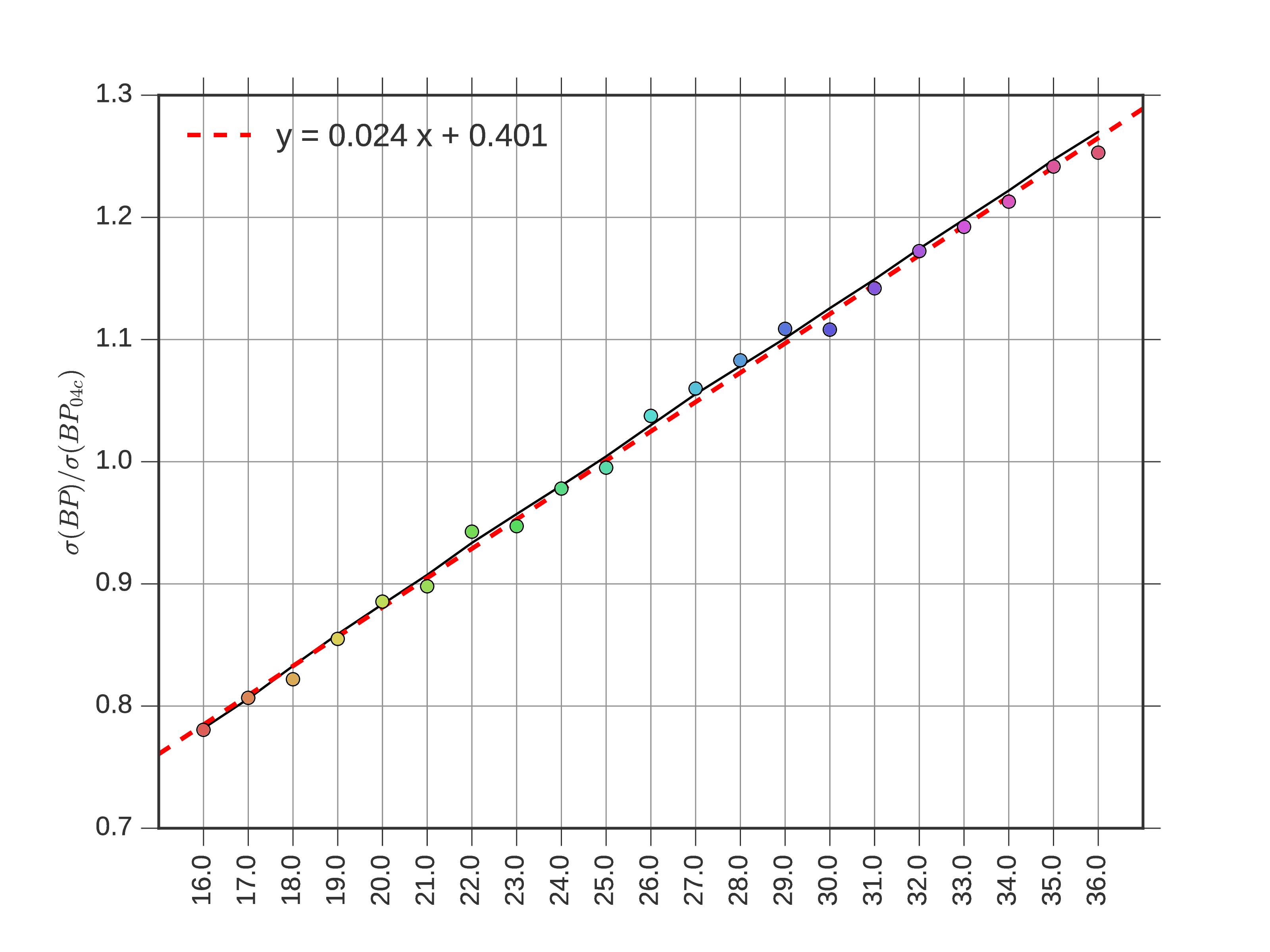
  In figure 5, we show the evolution of the noise bandpower std (normalized by the Pole hitmap case) as a function of field of view diameter.
  In this simple 1D approximation, going from a 28 degrees to a 35 degrees field of view enhances the noise std by 16%.

  

  ---

  
  

  3. Comparison with S4 power spectrum pipeline

  To check if our simple 1D model is a good approximation, in this section we compare some of the predictions with statistics derived from the final bandpowers obtained on simulated maps with the same DC04, DC04b and DC04c hitmaps, as already presented here.
  We produce ratios of the mean and std of the noise and signal bandpowers for 04b and 04c hitmaps over the stats for DC04 hitmaps. We also show effective \(f_{sky}\) of the noise and signal bandpowers and overlay the prediction of the simple 1D model.
  Looking at the TT statistics, it seems like our 1D models is a good tool to predict relative noise levels for different hitmaps.
  For the EE and BB statistics, there is a departure at low \(\ell\) that might be due to imperfections of the purification process, as discussed also in this recent posting.

  ---

  
  

  4. Comparison with the \(\sigma(r)\) results from the ML search and the Fisher framework (To be added).

  We saw in section 3 that this 1D model seems to be a fairly good tool to predict the statistics of the noise and signal bandpowers.
  Of course we are in fine interested in the effect on \(\sigma(r)\). The statistics of a given noise bandpower will not be related to this evolution in a trivial way, due to the effect of component separation and lensing.
  We can check using either the ML searches results on the DC04, DC04b and DC04c, as reported in this posting, or using the Fisher Framework for different field of views.

  In figure 7, we show the ratio of the \(\sigma(r)\) over the 3% circular hitmap case as a function of delensing, and overlayed with the ratio of the noise bandpowers predicted by the 1D model. In the case where there is no CMB signal: (\(A_L=0\) and \(r=0\)), it seems like the prediction could not be too bad, but it is not part of our standard runs.

  ---