| \(\sigma_r, (\times 10^{-3})\) | \(\Delta\) | \(\epsilon\) | |
|---|---|---|---|
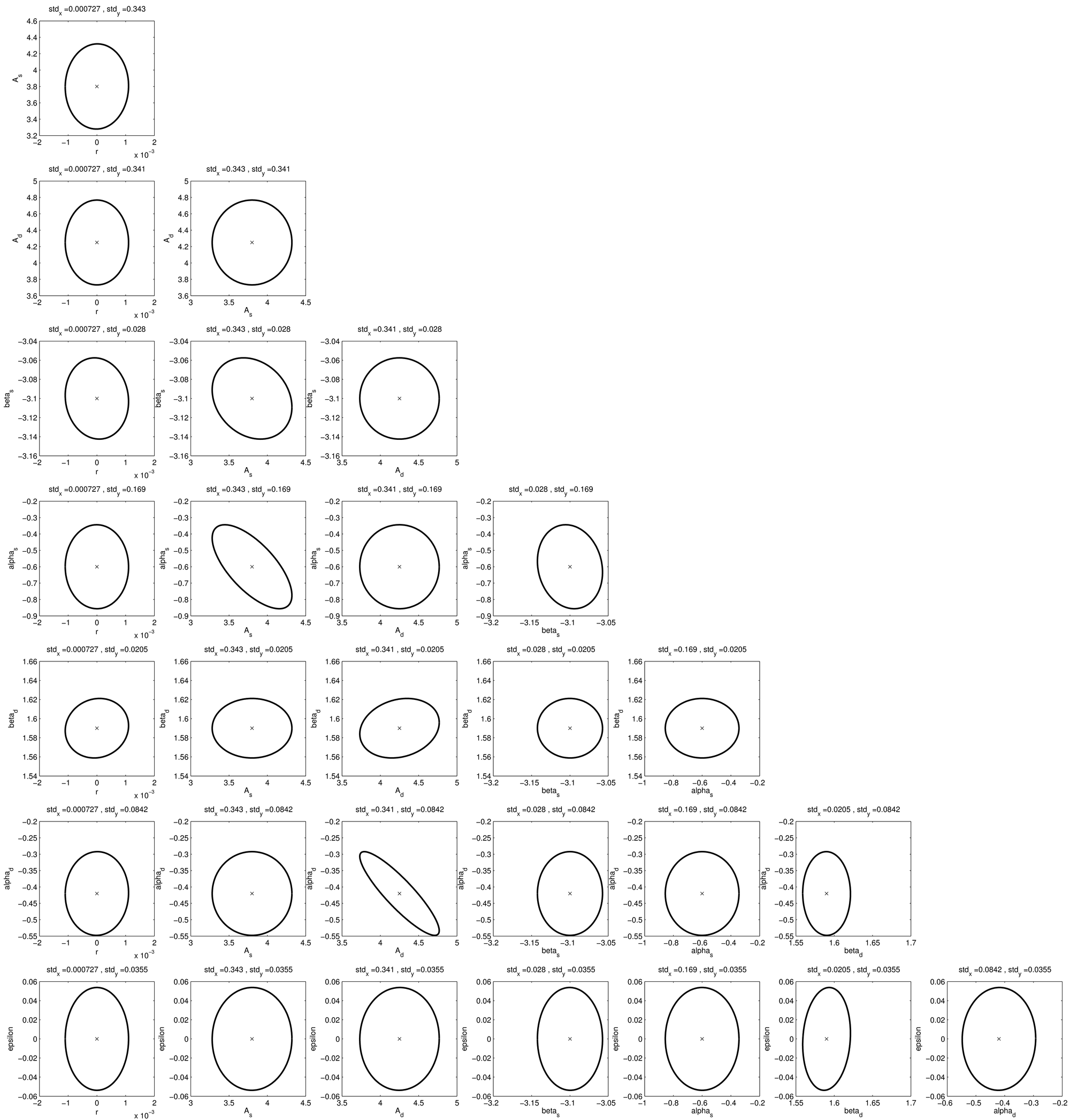
| No Systematics (Fisher Ellipses) | 0.727 | -- | -- |
| {\(X_i=0.05\), free}, {\(\alpha_i=0\), fixed} | 0.734 | 1.0% | 13.9% |
| {\(X_i=0.05\), free}, {\(\alpha_i=0\), free} | 0.771 | 6.1% | 35.3% |
| {\(X_i=0.05\), free, \(P(X)=0.075\)}, {\(\alpha_i=0\), free} | 0.742 | 2.1% | 20.4% |
Per-band irreducible residual (using \(r\) as template)
In this section I repeat the same procedure, except now I look at using a tensor signal with \(r=1\) as the systematic template. Our signal then has the following shape: \[S(\nu_1,\nu_2,l) = Y_i D^{tensor, r=1}_{l,i} \times\delta(\nu_1,\nu_2)\] Where we have one \(Y_i\) for each frequency. This means we now have 8 parameters instead of 16. It is clear that this case represents an evil scenario in which we have a systematic signal that looks exactly like \(r\) and our only saving grace is that we don't see it in the cross spectra. In this case, we would expect to see no constraining power from the auto spectra, and indeed we do see that!
| \(\sigma_r, (\times 10^{-3})\) | \(\Delta\) | \(\epsilon\) | |
|---|---|---|---|
| No Systematics (Fisher Ellipses) | 0.727 | -- | -- |
| {\(Y_i=0.05\), free} | 0.798 | 9.8% | 45.3% |
| {\(Y_i=0.05\), free, \(P(Y)=7.5\times 10^{-4}\)} | 0.743 | 2.2% | 21.1% |
| No Systematics (special case: No Auto-spectra) | 0.800 | 10.0% | 45.9% |
Common-mode irreducible residual construction
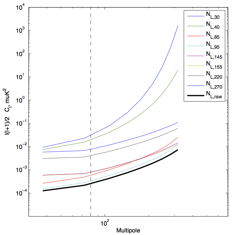
In comparison to the per-band residual, which only introduces a residual for the auto spectra, a common-mode residual is present in all auto and cross spectra, at the same amplitude, making it harder to separate from a signal like the CMB. This means only one parameter, and no Kronecker delta for the residual signal: \[S(\nu_1,\nu_2,l) = X N^{raw}_l \Big(\frac{l}{l_{pivot}}\Big)^\alpha\] where, for now, for a common template we use the raw noise of the experiment (combined across all bands, as plotted here): \[N^{raw}_l=\frac{1}{\sqrt{\sum^{n_{expt}}_i{1/N_{l,i}^2}}}\] The rest follows the same path. Calculating a Fisher Matrix with and without this common-mode residual yields:
| \(\sigma_r, (\times 10^{-3})\) | \(\Delta\) | \(\epsilon\) | \(\sigma_X\) | \(\sigma_\alpha\) | |
|---|---|---|---|---|---|
| No Systematics (Fisher Ellipses) | 0.727 | -- | -- | -- | -- |
| {\(X=0.05\), free}, {\(\alpha=0\), fixed} | 0.769 | 5.8% | 34.5% | 0.0423 | -- |
| {\(X=0.05\), free}, {\(\alpha=0\), free} | 1.582 | 117.6% | 193.3.6% | 0.2760 | 4.346 |
| {\(X=0.05\), free, \(P(X)=0.0290\)}, {\(\alpha=0\), free} | 0.742 | 2.1% | 20.4% | 0.0290 | 0.804 |
Common-mode irreducible residual (using \(r\) as template)
Similarly to the per-band residual, we also look at a common-mode residual that follows a tensor signal template. \[S(\nu_1,\nu_2,l) = Y D^{tensor, r=1}_{l,i}\] Where now we only have one parameter Y that tells us the amplitude of the injected signal in all auto and cross spectra. Such a signal is completely indistinguishable from \(r\) (i.e. fully degenerate with \(r\)), and therefore the degradation on \(\sigma_r\) is fully determined by the prior on \(Y\), as seen below.
| \(\sigma_r, (\times 10^{-3})\) | \(\Delta\) | \(\epsilon\) | \(\sigma_X\) | |
|---|---|---|---|---|
| No Systematics (Fisher Ellipses) | 0.727 | -- | -- | -- |
| {\(Y=0.05\), free, \(P(Y)=1.5\times 10^{-4}\)} | 0.742 | 2.1% | 20.4% | 0.00015 |
Biases on \(r\) due to an analysis blind to the form of residual systematics
With the above four cases in mind, we can set off to calculate the level of biases on \(r\) one would get if one were to inject these systematic signals into the data, and be completely agnostic to them in the model. To do this, I run a global Maximum Likelihood search over the default 8 parameters (r+foregrounds), before, and after the injection of systematics. The difference in the recovered \(r\) values between these cases tells us about the level of bias (i.e. what fraction of \(\sigma_r\)). I do this iteratively in order to figure what what signals will yield a bias on \(r\) that is close to 20% of \(\sigma_r\).
Recovered ML values before and after injection of per-band and common-mode systematics with the two templates described above. The \(X\) and \(Y\) values have been iteratively found to give us a bias equivalent to 20% of \(\sigma_r\).
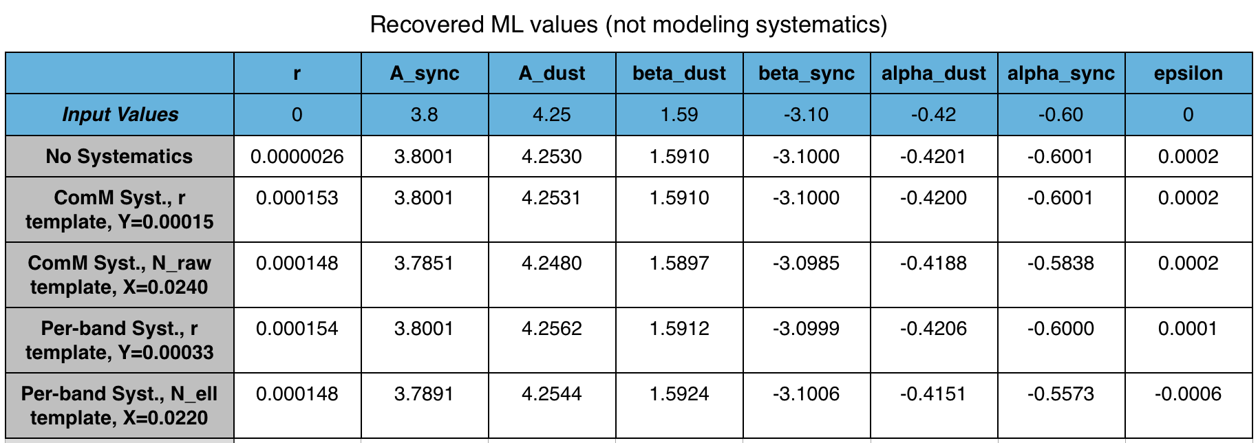
It is easy to note that the \(X\) and \(Y\) values here are lower than the values from obtained by including these parameters in the Fisher Model, and marginalizing over them. This is not surprising. The level of systematics we can tolerate will be lower when we have no information about the systematics in our maps than when we can model and marginalize over them.
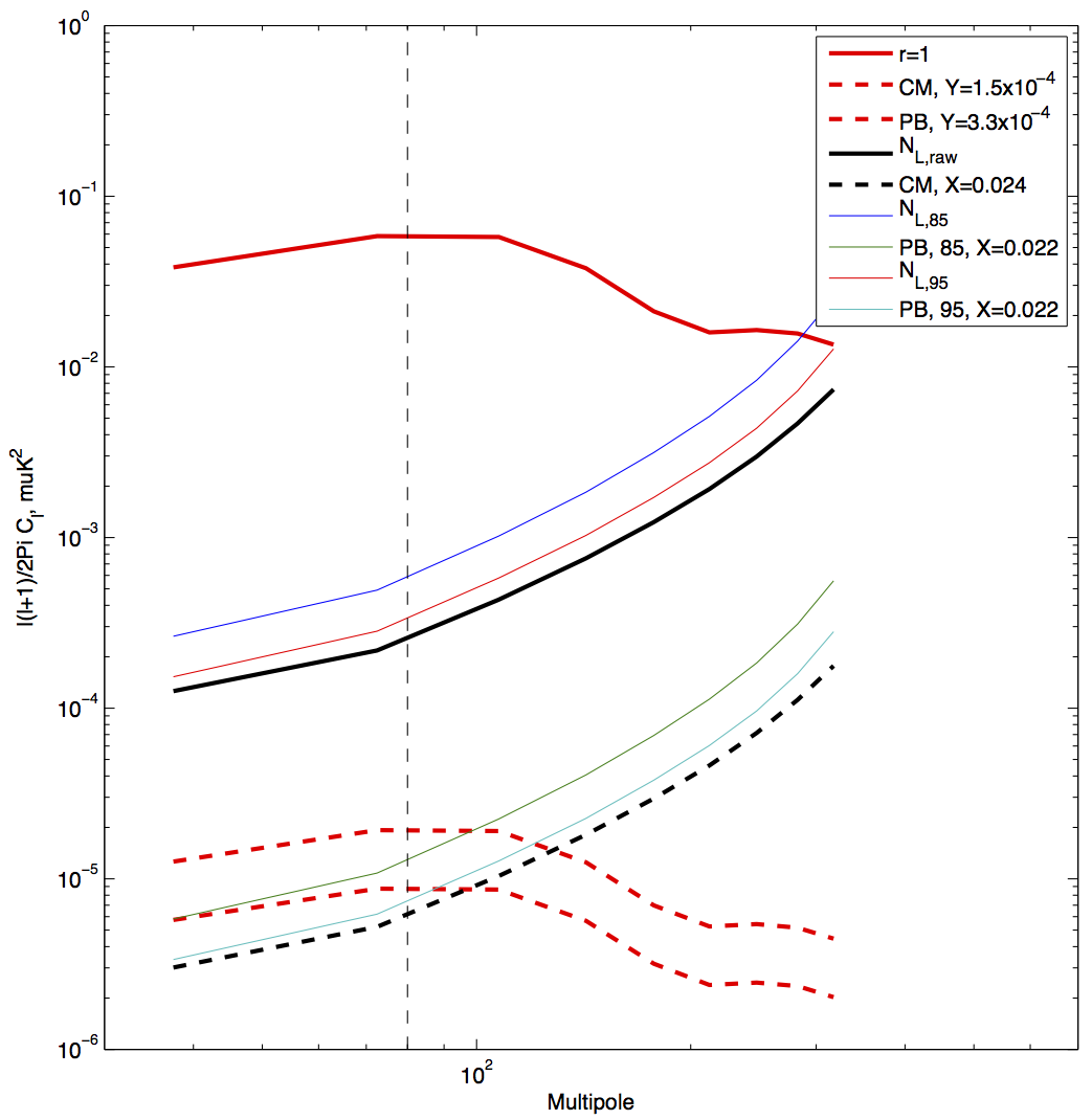
To derive measurement requirements from this analysis, we can look at the following plot, and read-off the power at \(l=80\) from the common-mode and per-band residuals. On this plot are the four level of systematics in the table above, that for each of the four cases yield a bias on \(r\) at the level of 20% of \(\sigma_r\), as well as the template shapes used for the systematics.
CM -- stands for Common-Mode; PB -- stands for Per-Band.
"Takeaways" Bullets:
- Each of the approaches (parametric Fisher and "blind" bias analyses, various ell forms for the contamination signal) suggest maximum levels for additive contamination to keep bias on "r" below delta(r) = 1.5e-4 (20% of current sigma(r) that are comparable, within a factor of 2-3. The "blind" levels are more stringent.
- We could summarize the measurement requirement for both per-band and common mode additive contamination as: "The sum of the unknown residual additive contamination from all systematic effects must be < 3 % of the final map noise for each survey band, and in the frequency-combined maps must be < 3% of the combined survey noise level, equivalent to 3 nK rms at \(l=80\)."
- DC 3 maps can be constructed with additive contamination added at the level of the measurement requirement by adding in extra scaled tensor components, both common mode and independent per band, for each of the 1000 realizations using tensors from on other realizations already on disk. Q: do we want both common-mode AND per-band to go into the same realizations? Is delta(r)=1.5e-4 large enough for this test?